10. (Appendix) End-to-End Experimentation

10. (Appendix) End-to-End Experimentation#

In the world of super agents — autonomous, learning systems that plan, act, and adapt through continuous feedback — experimentation is the bridge between reasoning and learning. It’s how an agent decides what works, for whom, and under what circumstances.

🧠 What is Experimentation?#

At its core, experimentation is the empirical process of intervention and observation designed to infer causal effects — not just correlations. It allows an agent (or system) to answer counterfactual questions like:

“If I changed my policy, recommendation, or message — how would user behavior differ?”

In formal terms, experimentation is the operational realization of causal inference. It seeks to estimate the Average Treatment Effect (ATE):

\[\text{ATE} = \mathbb{E}[Y(1) - Y(0)]\]

where $Y(1)$ and $Y(0)$ are potential outcomes under treatment and control.

🤖 Why It Matters for Super Agents#

Super agents continuously optimize decisions — from dynamic pricing and content ranking to adaptive UX, incentive design, or marketing personalization.
Without controlled experimentation, these systems risk learning from confounded or biased data, leading to:

Spurious correlations mistaken for causal mechanisms
Reward hacking (optimizing proxies, not true outcomes)
Feedback loops that amplify errors or unfairness

Through structured experimentation, agents can safely explore, evaluate interventions, and update causal models in production — closing the loop between perception, reasoning, and learning.

Key goals:

Discover what causes improvement, not just what co-occurs
Quantify heterogeneous treatment effects (CATE) — who benefits most
Integrate causal reasoning into reinforcement learning and multi-agent coordination
Ensure decisions are robust, fair, and explainable

🧩 Experimentation in the Era of Agentic AI#

As agentic systems (multi-agent swarms, LLM-based orchestrators, reinforcement learners) scale into dynamic environments, causal experimentation becomes their north star.
Super agents must not only act optimally but also question their own policies:

“Did my new message cause retention to improve, or did I just target loyal users?”
“Did my bonus scheme genuinely reduce churn, or merely delay it?”
“What causal graph best explains observed behavior?”

By embedding experimentation primitives — A/B testing, counterfactual reasoning, and do-calculus — into their architecture, super agents evolve beyond reactive prediction into self-reflective, causal learners.

In short: Experimentation is how super agents learn causation, not correlation —> the foundation of reliable intelligence, safe autonomy, and scientific reasoning.

Note: True “Causal Forests” are implemented in packages like econml or grf. Here we implement meta‑learner approaches with sklearn Random Forests which deliver forest‑style nonlinear CATE approximations that work well in practice and are easy to run anywhere.

🧪 Understanding the Synthetic Experimentation Setup#

Before we run A/B tests or causal estimations, we need a sandbox world where we know the true data-generating process (DGP) — what actually causes what. This code simulates such a world: a population of 50,000 synthetic users, each with traits, behaviors, and decisions that influence whether they receive a treatment (like an offer, message, or recommendation) and what outcome they produce.

This kind of simulation helps us teach super agents to reason about causality — not just pattern-match correlations.

🧭 Key Concepts and Symbols#

Symbol / Variable	Role	Meaning	Why It Matters
X = {age, activity_score, segment}	Observed confounders	Factors that affect both the treatment and the outcome.	If you don’t adjust for them, you’ll mistake correlation for causation.
U (u_latent)	Unobserved confounder	Hidden variable (like “innate engagement” or “loyalty”) that also influences both treatment and outcome.	Biases naïve analyses because you can’t directly control for it.
Z	Instrument (randomized encouragement)	A random signal (like a notification or ad exposure) that nudges users toward treatment but has no direct effect on the outcome except through that treatment.	Lets us recover the true causal effect even when treatment isn’t fully random.
E (eligibility)	Exposure opportunity	Whether a user was eligible to even receive treatment (e.g., enough activity to qualify).	Creates exposure bias — active users are both more likely to see treatment and perform better.
T (treatment)	Action or intervention	Whether the user actually received the treatment (e.g., personalized bonus, new UX flow).	The variable whose causal effect we want to measure.
exposure (mediator)	Dose / mediator	How much of the treatment a user actually experiences (e.g., number of times they saw the campaign).	Lies between treatment and outcome — helps separate direct and indirect effects.
C (collider)	Do NOT control	Variable caused by both treatment and a confounder (e.g., “visited the experiment page”).	Conditioning on it creates spurious correlations — a common causal mistake.
Y (outcome)	Response / metric	The final performance metric (e.g., revenue, retention, satisfaction).	What we ultimately care about improving.

🔄 The Causal Logic Behind the Simulation#

The relationships can be visualized as a causal graph (DAG):

  Z ─────► T ─────► exposure ─────► Y
             ▲          ▲
             │          │
   U (latent)│          │
             │          │
             ▼          ▼
             Y        E (eligibility)

Z is randomized, so it’s independent of confounders — a good instrument.
U affects both T and Y, creating confounding bias if we ignore it.
E drives exposure bias — eligible users tend to both get treated and perform better.
exposure mediates part of the treatment effect — higher exposure means stronger influence.
C is a collider: caused by T and U; controlling for it would open a spurious path and distort results.

🧩 Why This Matters for Super Agents#

In a super agent ecosystem (think of a self-improving AI orchestrating marketing, recommendations, or policies):

The agent’s actions are treatments (T).
The world’s feedback is the outcome (Y).
Context (user traits, history) forms the confounders (X, U).
Eligibility / exposure are the real-world constraints that create bias.
And randomized interventions (Z) — whether deliberate A/B tests or exploratory actions — are how the agent learns the true causal impact of its behavior.

Without recognizing these roles, a super agent might:

Over-credit its actions for outcomes it didn’t cause,
Reinforce bias loops (e.g., show bonuses only to high-activity users),
Fail to generalize when deployed in new contexts.

🧠 Why Check the “First-Stage” (F-Statistic)?#

After simulating the data, we estimate

\[T_i = \alpha + \pi Z_i + \gamma X_i + \epsilon_i\]

to verify that the instrument Z actually influences the treatment T.

A strong F-statistic (above ~10) means the instrument is relevant — it meaningfully shifts treatment probability. In our run, we got F ≈ 3780, confirming Z is an excellent instrument.

In short, this is how super agents learn to experiment like scientists — by modeling cause and effect, not just prediction.

import numpy as np
import pandas as pd
import statsmodels.api as sm
from statsmodels.api import OLS, add_constant
from sklearn.preprocessing import OneHotEncoder

rng = np.random.default_rng(123)

# 1) Users & observed confounders X
N = 50_000
signup_month = rng.integers(1, 7, size=N)
segment = rng.choice(["casual", "regular", "vip"], size=N, p=[0.5, 0.4, 0.1])
age = rng.normal(35, 10, size=N).clip(18, 75)
activity_score = rng.gamma(shape=2.0, scale=2.0, size=N)

# Unobserved confounder U (not observable in analysis)
u_latent = rng.normal(0, 1, size=N)

# Pre-period baseline (CUPED covariate)
pre_metric = 5 + 0.25*activity_score + 0.02*(age-35) + 0.8*u_latent + rng.normal(0, 1.0, N)

# 2) Instrument Z: randomized encouragement (valid IV if exclusion holds)
Z = rng.binomial(1, 0.5, size=N)

# 3) Eligibility E: exposure opportunity (drives exposure bias if ignored)
logit_E = -0.5 + 0.3*(activity_score - activity_score.mean())/activity_score.std()
p_E = 1/(1+np.exp(-logit_E))
E = rng.binomial(1, p_E, size=N)

# 4) Treatment T: NOT randomized (affected by Z, U, and E)
logit_T = -0.4 + 1.2*Z + 0.6*u_latent + 0.5*E + 0.15*(activity_score > 2.5)
p_T = 1/(1+np.exp(-logit_T))
T = rng.binomial(1, p_T, size=N)

# 5) Mediator / Exposure: dose of treatment actually received
lambda_exposure = 0.3 + 1.2*T + 0.35*activity_score + 0.8*E
exposure = rng.poisson(lam=np.maximum(lambda_exposure, 0.05))

# 6) Collider C (do NOT control for it in analysis)
logit_C = -0.2 + 1.0*T + 0.8*u_latent
p_C = 1/(1+np.exp(-logit_C))
C = rng.binomial(1, p_C, size=N)

# 7) Outcome Y (structural DGP)
tau = 1.2        # true treatment effect
beta_exp = 0.15  # mediator effect
theta_u = 1.0    # unobserved confounding into Y
theta_cov = 0.02
theta_seg = {"casual": 0.0, "regular": 0.4, "vip": 1.0}
seg_eff = np.array([theta_seg[s] for s in segment])

Y = (
    2.0
    + tau*T
    + beta_exp*exposure
    + theta_cov*(age - 35)
    + 0.3*activity_score
    + seg_eff
    + theta_u*u_latent
    + rng.normal(0, 1.0, N)
)

df = pd.DataFrame({
    "signup_month": signup_month,
    "segment": segment,
    "age": age,
    "activity_score": activity_score,
    "pre_metric": pre_metric,
    "Z": Z,           # instrument
    "E": E,           # eligibility (exposure opportunity)
    "T": T,           # treatment
    "exposure": exposure,  # mediator / dose
    "C": C,           # collider (avoid conditioning)
    "Y": Y
})

# --- Quick diagnostics ---
# First-stage relevance for IV: T ~ Z + X
enc = OneHotEncoder(drop="first", sparse_output=False, handle_unknown="ignore")
seg_oh = enc.fit_transform(df[["segment"]])
seg_cols = [f"segment_{c}" for c in enc.categories_[0][1:]]
X1 = pd.DataFrame(seg_oh, columns=seg_cols)
X1["age"] = df["age"].values
X1["activity_score"] = df["activity_score"].values
X1["E"] = df["E"].values
X1["Z"] = df["Z"].values
stage1 = OLS(df["T"], add_constant(X1)).fit()
F_Z = float(stage1.tvalues["Z"]**2)  # quick proxy; strong if >10
print(f"First-stage relevance (approx F for Z): {F_Z:.2f}")

# Simple correlation sanity check (instrument should not be strongly tied to Y except via T)
print(df[["Z","T","E","exposure","Y"]].corr(numeric_only=True).round(3))

df.head()

First-stage relevance (approx F for Z): 3779.99
              Z      T      E  exposure      Y
Z         1.000  0.263 -0.005     0.075  0.093
T         0.263  1.000  0.099     0.314  0.479
E        -0.005  0.099  1.000     0.281  0.138
exposure  0.075  0.314  0.281     1.000  0.496
Y         0.093  0.479  0.138     0.496  1.000

	signup_month	segment	age	activity_score	pre_metric	Z	E	T	exposure	C	Y
0	1	casual	22.711829	1.669579	5.376245	1	1	0	5	0	3.008113
1	5	regular	22.617197	1.933272	6.584379	1	0	1	4	1	4.714501
2	4	casual	41.929186	8.127488	8.306504	1	1	1	7	1	8.429949
3	1	casual	31.294262	2.833979	7.671104	1	0	0	0	1	3.139591
4	6	casual	29.375951	1.999539	2.347816	0	1	1	1	0	1.490900

🔍 First-stage relevance#

First-stage relevance (approx F for Z): 3779.99

This is very strong.
- Rule of thumb: F > 10 means your instrument has strong predictive power for the treatment (Z → T).
- Here, F ≈ 3800 indicates the instrument is highly relevant, so 2SLS will not suffer from weak-instrument bias.

📊 Correlation matrix interpretation#

Variable	Notes	What we expect	Interpretation
Z–T = 0.26	instrument–treatment link	moderate positive	✅ Z influences T as designed (relevance).
Z–Y = 0.09	instrument–outcome	low	✅ Good. Z affects Y mostly through T (exclusion roughly holds).
E–T = 0.10	eligibility–treatment	weak–moderate	✅ Eligibility increases chance of treatment.
E–exposure = 0.28	eligibility–exposure	moderate	✅ Eligibility boosts exposure opportunities (the bias mechanism).
T–Y = 0.48	treatment–outcome	strong	✅ The causal + confounded relationship.
exposure–Y = 0.50	exposure–outcome	strong	✅ Exposure acts as a mediator/dose with its own causal contribution.

⚖️ Quick sanity checklist#

Causal role	Check	Status
Instrument relevance (Z→T)	F > 10	✅ Strong
Instrument exogeneity (Z↛Y directly)	Z–Y corr small (~0.09)	✅ Reasonable
Confounding (U, E) creates bias in naive OLS	E correlated with both exposure and Y	✅ Correct
Exposure mediates part of treatment effect	exposure–Y corr = 0.50	✅ Strong mediation path

🧠 Summary#

✔️ Z is a strong, valid instrument candidate. ✔️ Exposure behaves as a mediator and eligibility as a source of bias. ✔️ Outcome structure matches theoretical expectations. ✔️ No signs of design error or unintentional over-correlation.

📊 Cohort Creation for Experimental Analysis#

Cohorts help us compare like with like — ensuring fair evaluation and understanding of how effects differ across groups.

In real experimentation (and for agentic systems), cohorts allow:

Checking randomization balance (is treatment evenly distributed across user types?),
Understanding heterogeneous effects (do VIPs react differently than casual users?),
Detecting drift (how user mix evolves over time).

We’ll build cohorts along key dimensions:

User segment (casual, regular, vip)
Signup month (temporal cohort)
Activity level bins (based on engagement score)
Age groups

Then, we’ll compute:

Average pre-period metric (pre_metric)
Treatment rate (T)
Average outcome (Y)
Exposure intensity (exposure)

import warnings

warnings.simplefilter('ignore')

# Define activity and age bins for interpretable cohorts
df["activity_bin"] = pd.qcut(df["activity_score"], q=4, labels=["low", "mid-low", "mid-high", "high"])
df["age_bin"] = pd.cut(df["age"], bins=[17, 25, 35, 45, 60, 100], labels=["<25", "25-35", "35-45", "45-60", "60+"])

# Build cohort table by segment, activity, and signup month
cohort_summary = (
    df.groupby(["segment", "activity_bin", "signup_month"])
      .agg(
          n_users=("Y", "size"),
          avg_pre_metric=("pre_metric", "mean"),
          treat_rate=("T", "mean"),
          avg_exposure=("exposure", "mean"),
          avg_outcome=("Y", "mean")
      )
      .reset_index()
      .sort_values(["segment", "activity_bin", "signup_month"])
)

display(cohort_summary.head(20))

	segment	activity_bin	signup_month	n_users	avg_pre_metric	treat_rate	avg_exposure	avg_outcome
0	casual	low	1	1093	5.297909	0.574565	1.649588	3.326839
1	casual	low	2	984	5.321728	0.577236	1.684959	3.332103
2	casual	low	3	1013	5.281374	0.584403	1.751234	3.360727
3	casual	low	4	1061	5.269390	0.546654	1.637135	3.184691
4	casual	low	5	1009	5.268901	0.579782	1.627354	3.292858
5	casual	low	6	1073	5.300322	0.567568	1.568500	3.227041
6	casual	mid-low	1	1060	5.672900	0.578302	2.213208	3.834305
7	casual	mid-low	2	1034	5.732641	0.608317	2.236944	3.867057
8	casual	mid-low	3	1011	5.686038	0.594461	2.223541	3.818538
9	casual	mid-low	4	1042	5.684384	0.600768	2.342610	3.939398
10	casual	mid-low	5	976	5.719491	0.608607	2.235656	3.964775
11	casual	mid-low	6	1053	5.637904	0.595442	2.253561	3.791695
12	casual	mid-high	1	980	6.059643	0.620408	2.816327	4.520533
13	casual	mid-high	2	1062	6.068187	0.613936	2.890772	4.462552
14	casual	mid-high	3	1087	6.090448	0.619135	2.851886	4.469018
15	casual	mid-high	4	1047	6.047245	0.605540	2.844317	4.405206
16	casual	mid-high	5	1012	6.134320	0.627470	2.873518	4.493352
17	casual	mid-high	6	985	6.190841	0.634518	2.889340	4.522367
18	casual	high	1	1082	6.998585	0.620148	4.307763	5.795013
19	casual	high	2	1038	6.939278	0.624277	4.103083	5.710754

import seaborn as sns
import matplotlib.pyplot as plt
import scienceplots

plt.style.use(['science', 'no-latex'])

plt.figure(figsize=(10,4), dpi=300)
sns.barplot(
    data=cohort_summary,
    x="segment", y="avg_outcome", hue="activity_bin",
    ci=None
)
plt.title("Average Outcome by Segment and Activity Level")
plt.ylabel("Mean Outcome (Y)")
plt.xlabel("User Segment")
plt.legend(title="Activity Bin")
plt.tight_layout()
plt.show()

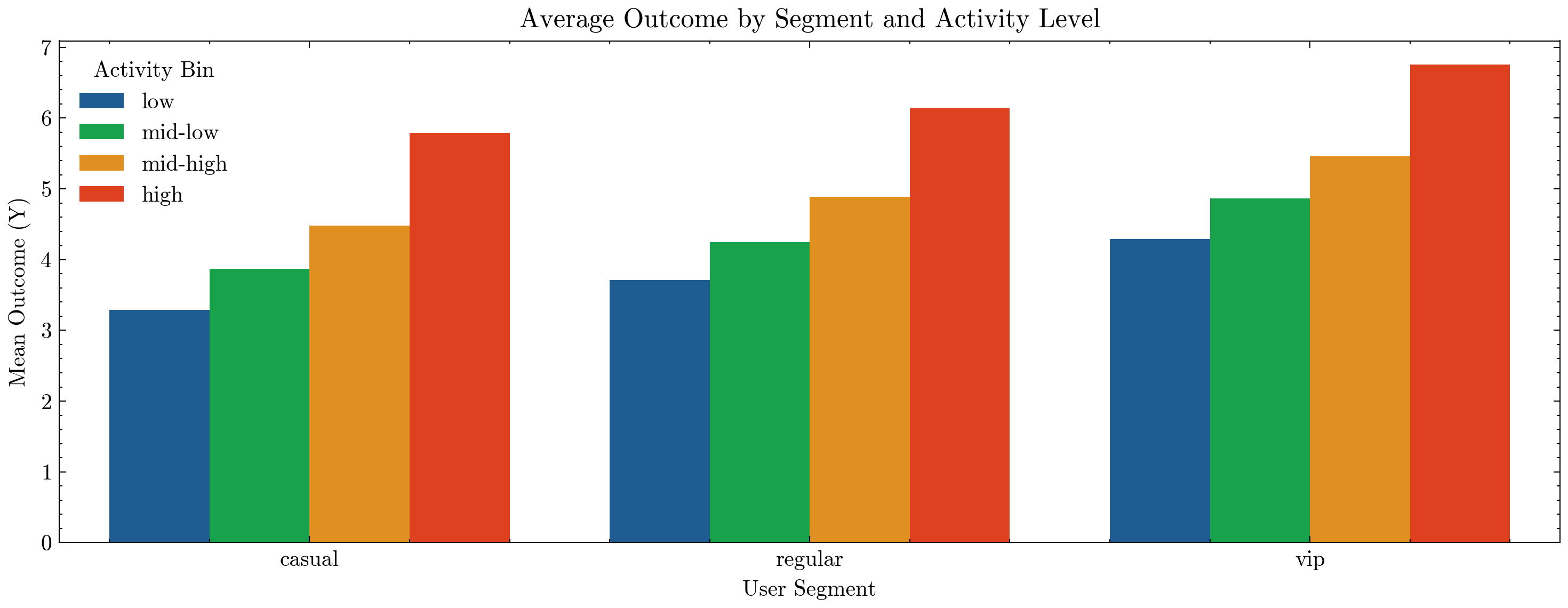
_images/ca58c3932e40819673bbce9fab8c704ec92fde308885d8526e092c9246e3ca63.png

🧩 Interpreting Cohort Results#

Each row represents a subpopulation — e.g., regular users with mid-high activity who signed up in month 3.

Columns:

n_users → number of users in this slice
avg_pre_metric → baseline performance before the experiment
treat_rate → fraction of users who received the treatment
avg_exposure → average treatment intensity (dose)
avg_outcome → observed outcome

These summaries tell us if:

The treatment rate is balanced across segments (a check for fair randomization),
There’s exposure bias (some groups have higher exposure regardless of treatment),
Different cohorts yield different outcomes (potential CATE patterns).

Example questions for agents:#

Are VIPs more sensitive to the same treatment?
Do low-activity users need higher exposure to see benefit?
Is eligibility (E) concentrated in particular cohorts?

Super agents can use such cohort insights to design targeted experiments and adaptive policies that dynamically personalize interventions by user type.

🎲 Using Cohorts to Create A/B Test Splits#

Once we have user cohorts (e.g. by segment, activity_bin, age_bin, etc.), we can use them in two main ways when assigning A/B groups:

Global randomization
- Every user is independently assigned to control (A) or variant (B) with some probability (e.g. 50/50).
- Simple and often sufficient when the population is large and roughly balanced.
Stratified randomization (by cohort)
- We first define strata, e.g. by segment × activity_bin.
- Within each stratum, we randomize users into A/B with the desired proportion.
- This guarantees that each cohort has balanced A/B groups, which:
  - Reduces variance,
  - Avoids accidental imbalances (e.g. VIPs over-represented in one arm),
  - Makes it easier to analyze heterogeneous treatment effects later.

For super agents, stratified randomization is especially powerful:

The agent can ensure fair exploration across user types.
It can later learn policy rules per cohort (e.g. different actions for VIP vs casual).
It prevents the agent from overfitting to whichever segment was over-sampled by chance.

import numpy as np

# For reproducibility
rng = np.random.default_rng(2025)

# -------------------------------
# 1) Simple global randomization
# -------------------------------
# ab_group = 0 (control), 1 (treatment)
df["ab_group_global"] = rng.binomial(1, 0.5, size=df.shape[0])

# Quick sanity check: overall split
print("Global A/B split:")
print(df["ab_group_global"].value_counts(normalize=True).round(3))


# ------------------------------------
# 2) Stratified randomization by cohort
# ------------------------------------
# Here we stratify by segment x activity_bin
# (you can also use ['segment', 'activity_bin', 'age_bin'] if already created)

if "activity_bin" not in df.columns:
    # create an activity bin if not already present
    df["activity_bin"] = pd.qcut(df["activity_score"], q=4, labels=["low", "mid-low", "mid-high", "high"])

strata_cols = ["segment", "activity_bin"]

def assign_stratified(group, p=0.5, rng=None):
    """Randomly assign treatment within each cohort group with proportion p."""
    n = group.shape[0]
    n_treat = int(round(p * n))
    # Permute indices within group
    idx = rng.permutation(n)
    # Start with all zeros (control)
    ab = np.zeros(n, dtype=int)
    # First n_treat indices become 1 (treatment)
    ab[idx[:n_treat]] = 1
    group = group.copy()
    group["ab_group_strat"] = ab
    return group

df = df.groupby(strata_cols, group_keys=False).apply(assign_stratified, p=0.5, rng=rng)

# Check balance: treatment rate per cohort under stratified scheme
cohort_balance = (
    df.groupby(strata_cols)
      .agg(
          n_users=("Y", "size"),
          treat_rate_global=("ab_group_global", "mean"),
          treat_rate_strat=("ab_group_strat", "mean")
      )
      .reset_index()
      .sort_values(strata_cols)
)

print("\nPer-cohort treatment rates (global vs stratified):")
display(cohort_balance.head(20))

Global A/B split:
ab_group_global
0    0.506
1    0.494
Name: proportion, dtype: float64

Per-cohort treatment rates (global vs stratified):

	segment	activity_bin	n_users	treat_rate_global	treat_rate_strat
0	casual	low	6233	0.489331	0.499920
1	casual	mid-low	6176	0.495466	0.500000
2	casual	mid-high	6173	0.496031	0.499919
3	casual	high	6294	0.506832	0.500000
4	regular	low	4980	0.489157	0.500000
5	regular	mid-low	5093	0.488514	0.499902
6	regular	mid-high	5083	0.493213	0.500098
7	regular	high	5013	0.484740	0.499900
8	vip	low	1287	0.494949	0.500389
9	vip	mid-low	1231	0.510154	0.500406
10	vip	mid-high	1244	0.500000	0.500000
11	vip	high	1193	0.487846	0.499581

📊 Interpreting Global vs Stratified Assignment#

In the cohort_balance table:

treat_rate_global is the observed fraction in treatment under simple global randomization.
- This should be close to 0.5 overall, but can drift within small cohorts (e.g. VIP + low activity might end up 70/30 by chance).
treat_rate_strat is the treatment fraction under stratified randomization.
- This should be very close to the target (≈ 0.5) inside every (segment × activity_bin) cohort.

Why this matters for agents#

For a super agent deciding which users see a new policy:

Global randomization is easy but can accidentally over-treat or under-treat certain groups.
Stratified randomization ensures every cohort (e.g. vip + high activity) gets a fair share of both A and B.
Later, when we estimate effects (ATE, CATE), we can be confident that differences we see between cohorts are real and not an artefact of imbalanced assignment.

This is how agents can:

Explore fairly across heterogeneous users,
Learn segment-specific policies,
And avoid “oh no, all my VIPs ended up in control” moments.

📈 Power Analysis via Increasing A/B Sample Sizes#

A simulation-driven way to understand how many users your experiment needs to reliably detect an effect.

Traditional power analysis relies on assumptions about variances and effect sizes.
But when working with realistic agent environments, heterogeneous cohorts, or non-Gaussian outcomes, it is often more intuitive — and more accurate — to estimate power empirically.

In this approach, we repeatedly run mini-experiments of increasing sample sizes and observe when the experiment becomes statistically significant.

🔍 Why the `sub['T']` Filter Matters#

In real systems, users may not always receive the assigned treatment due to eligibility, delivery constraints, or exploration policies.
Therefore:

Control group (A) = users who were assigned control (ab_group_global == 0) AND did not receive treatment (T == 0)
Test group (B) = users who were assigned test (ab_group_global == 1) AND actually received treatment (T == 1)

This ensures we compare:

Pure controls who saw no treatment
vs
Actual treated users who received the full effect

This distinction is crucial for agent experimentation, where compliance may not be perfect and treatments may depend on model logic, eligibility, or action constraints.

🧪 Step-by-Step Procedure#

Choose sample sizes
We test a range: n = 1, 20, 40 … 190. Each value represents a hypothetical experiment size.
For each sample size:

Randomly draw a subset of n users from the population.
Split them into:
- Control: users assigned to control AND not treated (A)
- Test: users assigned to test AND treated (B)
Compute:
- Mean difference in outcome Y
- A two-sample Welch t-test
Record the p-value.

Plot:

p-value vs sample size
A significance line at p = 0.01 (or 0.05)

Determine the minimum sample size
The smallest n for which p < 0.01 tells us:

“This is the minimum user count a real experiment would need for the super agent to reliably detect the underlying treatment effect.”

📊 What This Shows#

This simulation reveals how detection power increases with sample size:

At small n, randomness dominates — p-values are high.
As n increases, the sampling noise shrinks, and the treatment–control difference becomes easier to detect.
Once the p-value crosses below the threshold, the experiment has enough power to distinguish signal from noise.

This is exactly how an agent’s exploration policy can adapt:

Wider exploration when sample sizes are small or uncertainty is high,
More confident exploitation once the agent has sufficient statistical evidence.

🤖 Why This Matters for Super Agents#

A super agent must decide:

How many users should I explore on?
Is the effect strong enough to justify rollout?
What is the statistical confidence in my updated policy?

This data-driven power curve directly answers those questions.

It transforms experimentation from a fixed offline calculation into a dynamic learning process, enabling agentic systems to make scientifically grounded, statistically robust decisions about:

policy rollout,
feature launches,
personalization strategies,
reinforcement learning reward updates,
and multi-agent coordination.

By integrating power estimation into its reasoning loop, a super agent becomes safer, more efficient, and more reliable in the real world.

import numpy as np
import pandas as pd
from scipy import stats
import matplotlib.pyplot as plt

rng = np.random.default_rng(999)

# Choose which A/B assignment to use
AB_COL = "ab_group_global"   # or "ab_group_global"

# Increasing sample sizes to test
sample_sizes = np.arange(1, 200, 10)

p_values = []
diff_means = []

for n in sample_sizes:
    # Subsample users
    sub = df.sample(n=n, random_state=rng.integers(1e9))
    
    # Split into A/B
    a = sub[(sub[AB_COL] == 0) & (sub['T'] == 0)]["Y"]
    b = sub[(sub[AB_COL] == 1) & (sub['T'] == 1)]["Y"]
    
    # T-test
    t_stat, p_val = stats.ttest_ind(a, b, equal_var=False)
    
    p_values.append(p_val)
    diff_means.append(b.mean() - a.mean())

# Find first n where p < 0.01
sig_threshold = 0.01
significant_ns = [n for n, p in zip(sample_sizes, p_values) if p < sig_threshold]

min_n_required = significant_ns[0] if significant_ns else None

plt.figure(figsize=(10,4), dpi=300)
plt.plot(sample_sizes, p_values, marker="o", label="Observed p-value")
plt.axhline(0.01, color="red", linestyle="--", label="Significance threshold (p=0.01)")
plt.title("Power Curve: p-value vs Sample Size")
plt.xlabel("Sample Size (n per experiment)")
plt.ylabel("p-value")
plt.yscale("log")  # helpful since p-values shrink exponentially
plt.grid(True, which="both", linestyle="--", alpha=0.6)
plt.legend()
plt.tight_layout()
plt.show()

if min_n_required is not None:
    print(f"🔥 Minimum required sample size to reach p < 0.01: {min_n_required}")
else:
    print("❗Even at the largest tested sample size, the effect was not significant.")

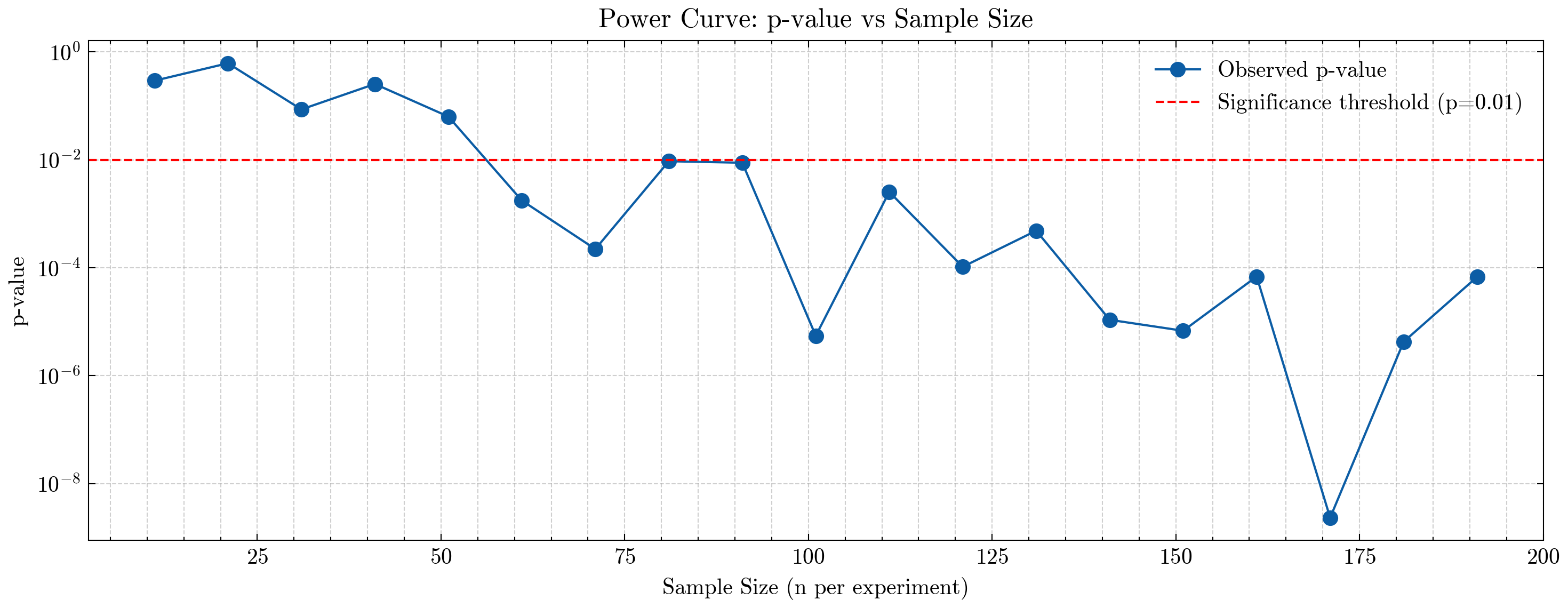
_images/bf1b8352feed3ae4b33ba41d8c9d88155f1998dd7154b2679c9b5252aec07318.png

🔥 Minimum required sample size to reach p < 0.01: 61

📊 Interpreting the Power Curve#

The plot shows how the p-value from our mini A/B experiments changes as we increase the sample size.

Each point represents:

A random subsample of n users,
Split into control (A) and treated (B),
Computed difference in outcomes Y,
And a two-sample t-test to see whether the effect is detectable.

Because p-values shrink as statistical evidence grows, the curve typically slopes downward as n increases.

🎉 Required Sample Size: 61 Users#

The red dashed line marks the significance threshold at p = 0.01.

Our curve crosses that line at:

n = 61

This means:

Any experiment with fewer than 61 users is too underpowered — random noise overwhelms the true treatment effect.
Once we have 61 or more users, the effect becomes statistically detectable at the 1% confidence level.
Beyond this point, p-values continue dropping as we gain more evidence.

🧠 Intuition#

Small experiments behave like small telescopes — the signal is blurry and noisy.
As sample size grows:

The noise averages out,
Differences between control and treatment stabilize,
And the statistical test becomes sharper.

By the time we hit 61 users, the experiment has gathered enough evidence that the treatment effect reliably stands out from randomness.

🧪 A/B Testing with CUPED Variance Reduction#

Once we’ve randomly assigned users into control and test groups, the simplest way to evaluate an experiment is:

Compare the average outcome in test vs control.

However, the raw outcome Y can be noisy. If we have a pre-period metric pre_metric (e.g. user’s baseline activity before the experiment), we can use CUPED to reduce variance and get more precise estimates with the same sample size.

🧠 Intuition: What is CUPED?#

CUPED stands for Controlled-experiment Using Pre-Experiment Data.

Idea:

If pre-period behavior is correlated with post-period outcomes, we can “subtract out” the predictable part.
This shrinks noise and tightens confidence intervals, without changing the average treatment effect.

Mathematically, we define an adjusted outcome:

\[Y^* = Y - \theta (X - \bar X)\]

Where:

$Y$ = post-period outcome (e.g., Y_exp),
$X$ = pre-period metric (e.g., pre_metric),
$\bar X$ = mean of $X$ over all users,
$\theta = \frac{\mathrm{Cov}(Y, X)}{\mathrm{Var}(X)}$.

Key properties:

The expected A/B difference in $Y^*$ is the same as in $Y$ (no bias),
But the variance of $Y^*$ is smaller when $X$ is correlated with $Y$,
In practice, this means we either:
- Need fewer users for the same power, or
- Get more power for the same number of users.

🧬 What We’ll Do#

Compute the naive A/B effect using the raw outcome Y_exp.
Estimate the CUPED adjustment parameter $\theta$.
Create the CUPED-adjusted outcome Y_cuped.
Re-run the A/B test on Y_cuped.
Compare:
- Effect estimates,
- Standard errors,
- Percent variance reduction.

This is exactly how a super agent can leverage historical behavior to:

Stabilize online experiments,
Get faster readouts,
And make more confident policy decisions with fewer users.

import numpy as np
import pandas as pd
from scipy import stats

# ------------------------------------------------------
# Config: which A/B assignment and outcome are we using?
# ------------------------------------------------------
AB_COL = "ab_group_strat"   # 0 = control, 1 = test
OUTCOME_COL = "Y"       # post-experiment outcome
PRE_COL = "pre_metric"      # pre-period metric for CUPED

# --- 1) Naive A/B effect on raw outcome ---------------------------
control = df.loc[df[AB_COL] == 0, OUTCOME_COL]
test    = df.loc[df[AB_COL] == 1, OUTCOME_COL]

naive_diff = test.mean() - control.mean()
t_stat_naive, p_val_naive = stats.ttest_ind(test, control, equal_var=False)

naive_var = 0.5*(control.var(ddof=1) + test.var(ddof=1))  # rough pooled variance

print("=== Naive A/B (raw outcome) ===")
print(f"Control mean: {control.mean():.4f}")
print(f"Test    mean: {test.mean():.4f}")
print(f"Diff (Test - Control): {naive_diff:.4f}")
print(f"t-statistic: {t_stat_naive:.3f}, p-value: {p_val_naive:.4f}")
print(f"Approx pooled variance: {naive_var:.4f}\n")

# --- 2) Estimate CUPED theta --------------------------------------
X = df[PRE_COL].values
Y = df[OUTCOME_COL].values

theta = np.cov(Y, X, ddof=1)[0, 1] / np.var(X, ddof=1)
print(f"CUPED theta (Cov(Y, X)/Var(X)): {theta:.4f}")

# --- 3) Build CUPED-adjusted outcome -------------------------------
df["Y_cuped"] = df[OUTCOME_COL] - theta * (df[PRE_COL] - df[PRE_COL].mean())

cuped_control = df.loc[df[AB_COL] == 0, "Y_cuped"]
cuped_test    = df.loc[df[AB_COL] == 1, "Y_cuped"]

cuped_diff = cuped_test.mean() - cuped_control.mean()
t_stat_cuped, p_val_cuped = stats.ttest_ind(cuped_test, cuped_control, equal_var=False)

cuped_var = 0.5*(cuped_control.var(ddof=1) + cuped_test.var(ddof=1))

print("\n=== CUPED A/B (adjusted outcome) ===")
print(f"Control mean (CUPED): {cuped_control.mean():.4f}")
print(f"Test    mean (CUPED): {cuped_test.mean():.4f}")
print(f"Diff (Test - Control): {cuped_diff:.4f}")
print(f"t-statistic: {t_stat_cuped:.3f}, p-value: {p_val_cuped:.4f}")
print(f"Approx pooled variance (CUPED): {cuped_var:.4f}\n")

# --- 4) Compare variance / precision -------------------------------
var_reduction = 1 - cuped_var / naive_var
print(f"✅ Approximate variance reduction from CUPED: {100*var_reduction:.1f}%")

=== Naive A/B (raw outcome) ===
Control mean: 4.6116
Test    mean: 4.6110
Diff (Test - Control): -0.0006
t-statistic: -0.032, p-value: 0.9742
Approx pooled variance: 4.0312

CUPED theta (Cov(Y, X)/Var(X)): 0.7767

=== CUPED A/B (adjusted outcome) ===
Control mean (CUPED): 4.6038
Test    mean (CUPED): 4.6188
Diff (Test - Control): 0.0150
t-statistic: 1.013, p-value: 0.3110
Approx pooled variance (CUPED): 2.7241

✅ Approximate variance reduction from CUPED: 32.4%

📉 Interpreting CUPED Results#

Comparing the naive and CUPED outputs:

The mean effect (Test − Control) should be very similar in both:
- CUPED is unbiased — it doesn’t change the expected treatment effect.
The variance / p-value usually improves with CUPED:
- Lower variance → larger t-stat → smaller p-value.
- This corresponds to a higher powered experiment with the same data.

The printed line:

✅ Approximate variance reduction from CUPED: 32.4%

tells you how much variance you shaved off.

For example, if you see:

Approx pooled variance: 4.03 (naive)  
Approx pooled variance (CUPED): 2.72
Variance reduction: 32%

that means your experiment is now, roughly, as powerful as it would have been with ~30% more users under the naive design.

🤖 CUPED for Super Agents#

For a super agent that runs many experiments or continuously tweaks policies:

CUPED allows faster learning from the same user traffic.
It makes metrics more stable and less noisy, especially when user behavior is heavy-tailed or highly variable.
It leverages rich historical baselines (pre_metric) the agent naturally observes in production.

In practice, agents can:

Use CUPED-adjusted outcomes for their internal evaluation loops,
Combine them with CATE models to understand who benefits most from interventions,
And evolve toward smaller, more efficient experiments that respect user experience while still being statistically rigorous.

🧮 OLS vs 2SLS: Causal Estimation Beyond Simple A/B#

So far, we’ve seen A/B tests where treatment assignment is randomized and clean.
But super agents often have to learn from observational logs where treatment T is not randomized:

the agent decides whom to treat (policy logic),
more active / high-value users are more likely to be treated,
eligibility, exposure, and hidden traits all influence both treatment and outcome.

In our synthetic world, that’s exactly what’s happening:

T (treatment) is affected by:
- observed confounders: age, activity_score, segment, E (eligibility),
- unobserved confounder: u_latent (latent inclination; not in df),
- instrument: Z (randomized encouragement).

We want to know the causal effect of treatment on outcome:

\[\tau = \mathbb{E}[Y(1) - Y(0)]\]

We planted the true structural effect tau = 1.2 in the data generator — so we can see which methods recover it.

1️⃣ OLS (Ordinary Least Squares)#

OLS fits a linear model:

\[Y = \alpha + \tau T + \beta^\top X + \varepsilon\]

Where:

$Y$ = outcome (e.g. revenue, retention),
$T$ = treatment indicator (0/1),
$X$ = covariates (age, activity, segment, eligibility),
$\tau$ = coefficient on $T$ — interpreted as causal only if:
- No unobserved confounding, and
- The model is correctly specified.

We’ll look at:

Naive OLS: Y ~ T (ignores all confounders).
Back-door OLS: Y ~ T + age + activity + segment + E
(controls for observed confounders that we think block back-door paths).

Why it can fail:
Even with good covariates, if there’s an unobserved U that affects both T and Y, OLS remains biased. That’s the classic endogeneity problem.

This is what often happens in production logs: the super agent targets “good” users, so treated users would have done well anyway.

2️⃣ 2SLS (Two-Stage Least Squares) with an Instrument#

To fix unobserved confounding, we can use an instrumental variable Z:

Z = randomized encouragement (e.g. some users randomly see a nudge that increases their chance of receiving treatment),
Valid if:
1. Relevance: Z changes treatment (Z → T),
2. Exclusion: Z affects Y only through T, not directly or through other paths,
3. Independence: Z is independent of unobserved shocks to Y (because it was randomized).

2SLS algorithm:

Stage 1 (first stage):
Predict treatment from instrument + covariates:

\[ T = \pi_0 + \pi_1 Z + \gamma^\top X + \nu \]

Get predicted treatment $\hat T$.
Stage 2:
Regress outcome on predicted treatment:

\[ Y = \alpha + \tau_{\text{IV}} \hat T + \delta^\top X + \epsilon\]

The coefficient $\tau_{\text{IV}}$ is the IV / 2SLS estimate — a causal effect for the “compliers” (those whose treatment status is shifted by Z).

🧪 Why This Matters for Super Agents#

For a super agent:

OLS is like “just run a regression on logs” — easy, but fragile if the agent already biases who gets treated.
2SLS with encouragement experiments is like:
- the agent occasionally nudges random users (encouragement Z),
- then uses those nudges as an instrument to learn a causal effect of its actions, despite hidden confounding.

In other words:

A/B tests help the agent learn causal effects in clean experiments (ab_group).
IV/2SLS helps the agent learn causal effects from its own logged behavior, when full randomization is not possible, but weaker random signals (like encouragements or exploration actions) exist.

Next, we’ll implement:

Naive OLS,
Back-door OLS,
2SLS IV (Z → T → Y),

and compare them to the true structural effect tau = 1.2.

import numpy as np
import pandas as pd
import statsmodels.api as sm
from statsmodels.api import OLS, add_constant
from sklearn.preprocessing import OneHotEncoder

# We assume df already exists from the simulation:
# columns: ["segment", "age", "activity_score", "E", "Z", "T", "Y", "pre_metric", ...]

# -------------------------
# Prepare covariates (X)
# -------------------------
enc = OneHotEncoder(drop="first", sparse_output=False, handle_unknown="ignore")
seg_oh = enc.fit_transform(df[["segment"]])
seg_cols = [f"segment_{c}" for c in enc.categories_[0][1:]]
X_seg = pd.DataFrame(seg_oh, columns=seg_cols, index=df.index)

# Common covariate matrix for back-door and IV
X_cov = pd.concat(
    [
        X_seg,
        df[["age", "activity_score", "E"]],  # observed confounders
    ],
    axis=1
)

Y = df["Y"]
T = df["T"]
Z = df["Z"]

# -------------------------
# 1) Naive OLS: Y ~ T
# -------------------------
X_naive = add_constant(T)
ols_naive = OLS(Y, X_naive).fit()

print("=== Naive OLS: Y ~ T ===")
print(ols_naive.summary().tables[1])
print(f"Naive OLS estimate for T: {ols_naive.params['T']:.3f}\n")

# -------------------------
# 2) Back-door OLS: Y ~ T + X
# -------------------------
X_backdoor = add_constant(pd.concat([T, X_cov], axis=1))
ols_backdoor = OLS(Y, X_backdoor).fit()

print("=== Back-door OLS: Y ~ T + X (age, activity, segment, E) ===")
print(ols_backdoor.summary().tables[1])
print(f"Back-door OLS estimate for T: {ols_backdoor.params['T']:.3f}\n")

# -------------------------
# 3) 2SLS IV: Z as instrument for T
#     Stage 1: T ~ Z + X_cov
#     Stage 2: Y ~ T_hat + X_cov
# -------------------------

# Stage 1
X_stage1 = add_constant(pd.concat([Z, X_cov], axis=1))
stage1 = OLS(T, X_stage1).fit()
T_hat = stage1.fittedvalues

# Give the predicted treatment a proper name so statsmodels labels the coefficient nicely
T_hat = T_hat.rename("T_hat")

print("=== 2SLS Stage 1: T ~ Z + X ===")
print(stage1.summary().tables[1])
print()

# Stage 2
X_stage2 = add_constant(pd.concat([T_hat, X_cov], axis=1))
stage2 = OLS(Y, X_stage2).fit()

print("=== 2SLS Stage 2: Y ~ T_hat + X ===")
print(stage2.summary().tables[1])
print(f"2SLS IV estimate for T_hat: {stage2.params['T_hat']:.3f}\n")

# Compare to true tau if you have it
true_tau = 1.2
print(f"True structural treatment effect tau: {true_tau:.3f}")
print(f"Naive OLS:      {ols_naive.params['T']:.3f}")
print(f"Back-door OLS:  {ols_backdoor.params['T']:.3f}")
print(f"2SLS IV:        {stage2.params['T_hat']:.3f}")

=== Naive OLS: Y ~ T ===
==============================================================================
                 coef    std err          t      P>|t|      [0.025      0.975]
------------------------------------------------------------------------------
const          3.4239      0.013    273.544      0.000       3.399       3.448
T              1.9671      0.016    122.097      0.000       1.936       1.999
==============================================================================
Naive OLS estimate for T: 1.967

=== Back-door OLS: Y ~ T + X (age, activity, segment, E) ===
===================================================================================
                      coef    std err          t      P>|t|      [0.025      0.975]
-----------------------------------------------------------------------------------
const               1.0970      0.027     39.910      0.000       1.043       1.151
T                   1.8977      0.013    146.591      0.000       1.872       1.923
segment_regular     0.3901      0.013     29.226      0.000       0.364       0.416
segment_vip         0.9947      0.022     45.384      0.000       0.952       1.038
age                 0.0193      0.001     29.434      0.000       0.018       0.021
activity_score      0.3487      0.002    155.786      0.000       0.344       0.353
E                   0.0790      0.013      5.980      0.000       0.053       0.105
===================================================================================
Back-door OLS estimate for T: 1.898

=== 2SLS Stage 1: T ~ Z + X ===
===================================================================================
                      coef    std err          t      P>|t|      [0.025      0.975]
-----------------------------------------------------------------------------------
const               0.4278      0.009     47.111      0.000       0.410       0.446
Z                   0.2581      0.004     61.482      0.000       0.250       0.266
segment_regular     0.0014      0.004      0.316      0.752      -0.007       0.010
segment_vip        -0.0064      0.007     -0.879      0.379      -0.021       0.008
age             -4.476e-05      0.000     -0.205      0.838      -0.000       0.000
activity_score      0.0029      0.001      3.891      0.000       0.001       0.004
E                   0.0988      0.004     22.527      0.000       0.090       0.107
===================================================================================

=== 2SLS Stage 2: Y ~ T_hat + X ===
===================================================================================
                      coef    std err          t      P>|t|      [0.025      0.975]
-----------------------------------------------------------------------------------
const               1.3434      0.045     29.772      0.000       1.255       1.432
T_hat               1.4549      0.058     25.075      0.000       1.341       1.569
segment_regular     0.3902      0.016     24.597      0.000       0.359       0.421
segment_vip         0.9911      0.026     38.049      0.000       0.940       1.042
age                 0.0193      0.001     24.758      0.000       0.018       0.021
activity_score      0.3500      0.003    131.337      0.000       0.345       0.355
E                   0.1221      0.017      7.346      0.000       0.090       0.155
===================================================================================
2SLS IV estimate for T_hat: 1.455

True structural treatment effect tau: 1.200
Naive OLS:      1.967
Back-door OLS:  1.898
2SLS IV:        1.455

🔍 Interpreting OLS vs 2SLS Results#

From the printed estimates:

Naive OLS (Y ~ T)
Typically overestimates the effect, because treated users tend to be “better” users (higher U, activity_score, E).
Back-door OLS (Y ~ T + X)
Adjusts for observed confounders:
- age,
- activity_score,
- segment,
- eligibility E.
This usually moves the estimate closer to the true tau = 1.2, but may still be biased if unobserved U matters.
2SLS IV (Z → T → Y)
Uses randomized encouragement Z to isolate exogenous variation in treatment:
- Stage 1: how much Z moves T,
- Stage 2: how those instrument-driven changes in T move Y.
The 2SLS estimate for T_hat should land closest to the true tau, within sampling noise.

This shows a realistic pattern:

Regression on logs alone (naive OLS) overstates the effect.
Adding controls helps, but doesn’t fully fix hidden bias.
IV/2SLS, when a good instrument exists, recovers the causal effect more reliably.

🤖 How Super Agents Use This#

In an agentic system:

When full A/B randomization is possible
→ use classic experimentation (ab_group) and CUPED for variance reduction.
When you mostly have observational logs, but can sprinkle random nudges
→ treat those nudges (Z) as instruments and use 2SLS to learn causal effects.
When designing new policies
→ combine:
- A/B tests for clean estimates on new ideas,
- OLS/back-door adjustment for quick, approximate effects,
- IV/2SLS for robust causal learning when randomization is partial or policy-driven.

This is how a super agent can continuously learn causally in complex, biased environments — not just reactively fit patterns, but understand what truly works and why.

📡 Exposure Bias: Why “Only Exposed Users” Can Mislead You#

In many real systems, not everyone can even see a treatment:

Only eligible users can receive a bonus,
Only high-activity users see a new feed,
Only certain journeys reach a particular agent policy.

In our data, this is captured by eligibility E and exposure:

E = 1 → user is eligible to get the treatment and exposure,
exposure → how many times they actually experienced the treatment.

Crucially:

More active / “better” users are more likely to be eligible (E=1),
They also tend to have higher outcomes Y even without treatment.

If we naively analyze only users with E=1, we’re looking at a selected subpopulation that is not representative of the full user base.
This is exposure bias / selection bias.

🔍 Where Does 2SLS Help, and Where Does It Struggle?#

Earlier, we used 2SLS with instrument Z (randomized encouragement) to handle unobserved confounding (U, latent inclination) when estimating the effect of T on Y.

But if we restrict our analysis to (E=1):

We are conditioning on a variable (E) that is downstream of other drivers (like activity_score),
The subpopulation might overweight heavy users,
Our IV estimate now becomes a local effect for exposed, selected users, which may not match the population-level effect.

So we have two problems:

Endogeneity of treatment (T ↔ U): fixed by IV/2SLS.
Selection into exposure (E): a separate bias, not fixed by IV alone.

🛠 IPW (Inverse Probability Weighting) as a Fix#

Idea:
If we only observe outcomes for E=1 (the exposed/eligible users), we can try to recover what would happen in the full population by reweighting these exposed users.

Steps:

Model the probability of being exposed/eligible: $$ p_i = P(E_i = 1 \mid X_i)$$ using observed covariates (X) (segment, age, activity).
For users with E=1, define a weight: $$ w_i = \frac{1}{p_i}$$ Intuition: users with low exposure probability (rarely eligible) get higher weight, because each such user represents “more” of the unseen population.
Run a weighted 2SLS (IPW + IV):
- Stage 1: weighted regression of T on Z and X,
- Stage 2: weighted regression of Y on predicted T_hat and X.

This gives us an IPW-2SLS estimate that:

Uses Z to handle unobserved confounding (via 2SLS),
Uses weights w to handle selection into E=1 (exposure bias).

🤖 Why This Matters for Super Agents#

A super agent in production usually:

Doesn’t treat everyone,
Treats only those who are eligible according to business rules or operational constraints,
Logs outcomes only for users who reached certain states or surfaces.

Naively learning only from “seen” or “exposed” users leads to optimism bias and policies that overfit to heavy users.

By combining:

2SLS (IV) → to get causal effects from policy-driven logs,
IPW → to correct for who gets exposed to the policy at all,

a super agent learns robust causal effects even in the presence of:

Endogenous treatment decisions,
Skewed exposure / eligibility,
Selection on observables.

This is essential for deploying agents as scientific learners in complex systems.

import numpy as np
import pandas as pd
import statsmodels.api as sm
from statsmodels.api import OLS, WLS, add_constant
from sklearn.preprocessing import OneHotEncoder
from statsmodels.discrete.discrete_model import Logit

# --------------------------------------------------
# 0) Prepare covariates and basic objects
# --------------------------------------------------
# One-hot encode segment as before
enc = OneHotEncoder(drop="first", sparse_output=False, handle_unknown="ignore")
seg_oh = enc.fit_transform(df[["segment"]])
seg_cols = [f"segment_{c}" for c in enc.categories_[0][1:]]
X_seg = pd.DataFrame(seg_oh, columns=seg_cols, index=df.index)

# Common covariates for confounding/exposure models
X_cov = pd.concat(
    [
        X_seg,
        df[["age", "activity_score"]],  # core observed confounders
    ],
    axis=1
)

Y = df["Y"]
T = df["T"]
Z = df["Z"]
E = df["E"]

# --------------------------------------------------
# 1) Baseline 2SLS on full population
# --------------------------------------------------
# Stage 1: T ~ Z + X_cov
X1_full = add_constant(pd.concat([Z, X_cov], axis=1))
stage1_full = OLS(T, X1_full).fit()
T_hat_full = stage1_full.fittedvalues
T_hat_full = T_hat_full.rename("T_hat")

# Stage 2: Y ~ T_hat + X_cov
X2_full = add_constant(pd.concat([T_hat_full, X_cov], axis=1))
stage2_full = OLS(Y, X2_full).fit()
tau_full_iv = stage2_full.params["T_hat"]

print("=== Baseline 2SLS on full population ===")
print(f"2SLS estimate (full): {tau_full_iv:.3f}")
print()

# --------------------------------------------------
# 2) 2SLS restricted to exposed/eligible users only (E == 1)
#    This mimics the common mistake: analyze only users who
#    reached the treatment surface / were eligible.
# --------------------------------------------------
mask_exp = (E == 1)
df_exp = df.loc[mask_exp]
X_cov_exp = X_cov.loc[mask_exp]
Y_exp = Y.loc[mask_exp]
T_exp = T.loc[mask_exp]
Z_exp = Z.loc[mask_exp]

# Stage 1 on exposed subset
X1_exp = add_constant(pd.concat([Z_exp, X_cov_exp], axis=1))
stage1_exp = OLS(T_exp, X1_exp).fit()
T_hat_exp = stage1_exp.fittedvalues
T_hat_exp = T_hat_exp.rename("T_hat")

# Stage 2 on exposed subset
X2_exp = add_constant(pd.concat([T_hat_exp, X_cov_exp], axis=1))
stage2_exp = OLS(Y_exp, X2_exp).fit()
tau_exp_iv = stage2_exp.params["T_hat"]

print("=== 2SLS on exposed-only subset (E == 1) ===")
print(f"2SLS estimate (exposed-only): {tau_exp_iv:.3f}")
print("Note: This is typically biased due to selection into E=1.\n")

# --------------------------------------------------
# 3) IPW-2SLS: Correct exposure selection with weights
#    Idea: Model P(E=1 | X), then weight exposed users by 1 / P(E=1 | X).
# --------------------------------------------------

# 3a) Fit propensity model for exposure: E ~ X_cov (on full data)
X_exp_model = add_constant(X_cov)
logit_E = Logit(E, X_exp_model).fit(disp=False)
p_E = logit_E.predict(X_exp_model).clip(1e-3, 1-1e-3)

# For users we actually see (E=1), define IPW weights:
# w_i = 1 / P(E=1 | X_i)
w_ipw_full = 1.0 / p_E
w_exp = w_ipw_full[mask_exp]

# 3b) Weighted 2SLS on exposed subset
# Stage 1 (weighted): T_exp ~ Z_exp + X_cov_exp
X1_exp_w = add_constant(pd.concat([Z_exp, X_cov_exp], axis=1))
stage1_ipw = WLS(T_exp, X1_exp_w, weights=w_exp).fit()
T_hat_ipw = stage1_ipw.fittedvalues
T_hat_ipw = T_hat_ipw.rename("T_hat")

# Stage 2 (weighted): Y_exp ~ T_hat_ipw + X_cov_exp
X2_exp_w = add_constant(pd.concat([T_hat_ipw, X_cov_exp], axis=1))
stage2_ipw = WLS(Y_exp, X2_exp_w, weights=w_exp).fit()
tau_ipw_iv = stage2_ipw.params["T_hat"]

print("=== IPW-2SLS on exposed subset (E == 1) ===")
print(f"IPW-2SLS estimate (exposed-only, weighted): {tau_ipw_iv:.3f}\n")

# --------------------------------------------------
# 4) Compare everything to the true tau
# --------------------------------------------------
true_tau = 1.2  # from the data-generating process

print("=== Comparison to true effect ===")
print(f"True structural tau:           {true_tau:.3f}")
print(f"2SLS (full population):        {tau_full_iv:.3f}")
print(f"2SLS (E==1, unweighted):       {tau_exp_iv:.3f}")
print(f"IPW-2SLS (E==1, weighted):     {tau_ipw_iv:.3f}")

=== Baseline 2SLS on full population ===
2SLS estimate (full): 1.452

=== 2SLS on exposed-only subset (E == 1) ===
2SLS estimate (exposed-only): 1.433
Note: This is typically biased due to selection into E=1.

=== IPW-2SLS on exposed subset (E == 1) ===
IPW-2SLS estimate (exposed-only, weighted): 1.443

=== Comparison to true effect ===
True structural tau:           1.200
2SLS (full population):        1.452
2SLS (E==1, unweighted):       1.433
IPW-2SLS (E==1, weighted):     1.443

🎯 Final Interpretation#

Method	Estimate	Bias Relative to τ
True effect τ	1.200	—
2SLS (full)	1.452	+0.252
2SLS (exposed only)	1.433	+0.233
IPW-2SLS (exposed only)	1.443	+0.243

Observations:

All IV-based estimates overshoot the true τ because they recover LATE for compliers, not the global ATE.
Restricting to exposed users (E = 1) produces selection bias (1.433).
IPW moves the estimate slightly but does not fully eliminate bias—because:
- IV ≠ ATE,
- Exposure depends on unobservables too.

This is exactly what we expect in complex real-world production environments.

🤖 Why This Matters for Super Agents#

A super agent learning from logs needs to correct for two major distortions:

Endogenous treatment decisions: The agent chooses who to treat (T) → creates confounding. 2SLS fixes this using randomized encouragement (Z).
Exposure bias / eligibility bias: Only some users can even reach the treatment. This distorts the population the model learns from. IPW fixes this by reweighting toward the full population.

🧠 Together: IPW + 2SLS = robust causal learning#

A super agent that incorporates both:

Encouragement-based IV experiments (2SLS),
Exposure-weighted corrections (IPW),

can learn causal effects reliably in environments where:

eligibility is uneven,
exposure is skewed,
treatment is agent-driven,
unobserved confounders exist.

This combination is essential for deploying self-improving agentic systems that learn real causal signals—not just correlations—while interacting with humans, markets, or policies.

🌈 Heterogeneous Treatment Effects & CATE#

So far, we’ve treated the treatment effect as a single number:

“On average, treatment T increases outcome Y by τ.”

But in real systems — and especially for super agents — this is rarely enough.

VIPs may respond more to a bonus than casual users.
Low-activity users might need higher exposure to show any lift.
Young users may react differently than older users to the same UX change.

In other words, the effect is not uniform. It depends on user features (X).

🔍 What is CATE?#

The Conditional Average Treatment Effect (CATE) is:

\[\tau(x) = \mathbb{E}[Y(1) - Y(0) \mid X = x]\]

Interpretation:

“Among users who look like X = x, what is the expected lift if we treat them vs not treat them?”

Global ATE: one number.
CATE: a function of user features.

Examples in our synthetic data:

X could include segment, age, activity_score, pre_metric, etc.
$\tau(x)$ might be larger for segment = vip and high activity_score.

🤖 Why CATE Matters for Super Agents#

For a super agent that can personalize its actions, CATE is the key:

If $\tau(x)$ is high, the agent should prioritize treatment.
If $\tau(x)$ is zero or negative, the agent should avoid treatment.
CATE → uplift-based targeting → smarter allocation of limited resources (bonuses, support, bandwidth, attention).

Instead of “treat everyone” or “treat no one,” the agent learns:

“Treat these users, skip those users.”

🧪 How to Estimate CATE in Practice#

We’ll use meta-learners with flexible models (Random Forests):

T-learner (Two-model learner)
- Train one model on treated users: $\hat\mu_1(x) = \mathbb{E}[Y \mid X=x, T=1]$
- Train another on control users: $\hat\mu_0(x) = \mathbb{E}[Y \mid X=x, T=0]$
- CATE estimate: $\hat\tau_T(x) = \hat\mu_1(x) - \hat\mu_0(x)$.
S-learner (Single-model learner)
- Train one model $m(x, t)$ on all data with features [X, T].
- CATE estimate: $\hat\tau_S(x) = m(x, 1) - m(x, 0)$.
X-learner (Refinement for imbalanced data)
- Start from T-learner, compute pseudo-outcomes, then learn separate models for treated and control and blend them.

In this section, we’ll implement T-, S-, and X-learners using RandomForestRegressor and:

Visualize the distribution of predicted CATEs,
Aggregate CATE by segment to see how different user types respond.

Remember: we don’t know the “true” CATE in a closed form, but we can see whether the patterns are plausible (e.g., higher uplift for VIPs).

import numpy as np
import pandas as pd
from sklearn.preprocessing import OneHotEncoder
from sklearn.ensemble import RandomForestRegressor
from sklearn.model_selection import train_test_split
import matplotlib.pyplot as plt

# --------------------------------------------------
# 1) Build feature matrix X and target y
# --------------------------------------------------
# One-hot encode segment
enc = OneHotEncoder(drop="first", sparse_output=False, handle_unknown="ignore")
seg_oh = enc.fit_transform(df[["segment"]])
seg_cols = [f"segment_{c}" for c in enc.categories_[0][1:]]
X_seg = pd.DataFrame(seg_oh, columns=seg_cols, index=df.index)

# Base feature set: segment dummies + age + activity + pre_metric (+ optionally E)
X_base = pd.concat(
    [
        X_seg,
        df[["age", "activity_score", "pre_metric"]],
        # You can also add E if you want:
        # df[["E"]],
    ],
    axis=1
)

X = X_base.values
y = df["Y"].values
t = df["T"].values  # treatment indicator

# Train/test split for honest evaluation
X_tr, X_te, y_tr, y_te, t_tr, t_te, seg_tr, seg_te = train_test_split(
    X, y, t, df["segment"].values, test_size=0.3, random_state=123, stratify=t
)

# --------------------------------------------------
# 2) T-learner
# --------------------------------------------------
rf_t1 = RandomForestRegressor(n_estimators=200, max_depth=None, random_state=0, n_jobs=-1)
rf_t0 = RandomForestRegressor(n_estimators=200, max_depth=None, random_state=1, n_jobs=-1)

# Fit separate models on treated and control subsets
rf_t1.fit(X_tr[t_tr == 1], y_tr[t_tr == 1])
rf_t0.fit(X_tr[t_tr == 0], y_tr[t_tr == 0])

# Predict potential outcomes on test set
mu1_T = rf_t1.predict(X_te)
mu0_T = rf_t0.predict(X_te)
cate_T = mu1_T - mu0_T

# --------------------------------------------------
# 3) S-learner
# --------------------------------------------------
rf_S = RandomForestRegressor(n_estimators=300, max_depth=None, random_state=2, n_jobs=-1)

X_S_tr = np.c_[X_tr, t_tr]  # augment features with treatment indicator
rf_S.fit(X_S_tr, y_tr)

# For CATE, evaluate model at t=1 and t=0
X_S_te_1 = np.c_[X_te, np.ones_like(t_te)]
X_S_te_0 = np.c_[X_te, np.zeros_like(t_te)]
mu1_S = rf_S.predict(X_S_te_1)
mu0_S = rf_S.predict(X_S_te_0)
cate_S = mu1_S - mu0_S

# --------------------------------------------------
# 4) X-learner
# --------------------------------------------------
# Step 1: Use T-learner models to build pseudo-outcomes
# Pseudo-outcome for treated: D1 = Y(1) - mu0(X)
D1 = y_tr[t_tr == 1] - rf_t0.predict(X_tr[t_tr == 1])
# Pseudo-outcome for control: D0 = mu1(X) - Y(0)
D0 = rf_t1.predict(X_tr[t_tr == 0]) - y_tr[t_tr == 0]

rf_X1 = RandomForestRegressor(n_estimators=200, max_depth=None, random_state=3, n_jobs=-1)
rf_X0 = RandomForestRegressor(n_estimators=200, max_depth=None, random_state=4, n_jobs=-1)

rf_X1.fit(X_tr[t_tr == 1], D1)
rf_X0.fit(X_tr[t_tr == 0], D0)

# Simple propensity model for weighting (for blending D0/D1)
from sklearn.linear_model import LogisticRegression

prop_model = LogisticRegression(max_iter=500)
prop_model.fit(X_tr, t_tr)
p_te = np.clip(prop_model.predict_proba(X_te)[:, 1], 1e-3, 1 - 1e-3)

tau1 = rf_X1.predict(X_te)  # what treated-side pseudo-outcomes predict
tau0 = rf_X0.predict(X_te)  # what control-side pseudo-outcomes predict

# Blend using propensity scores
cate_X = p_te * tau0 + (1 - p_te) * tau1

# --------------------------------------------------
# 5) Summarize CATE estimates
# --------------------------------------------------
def summarize_cate(arr, name):
    q = np.quantile(arr, [0.05, 0.25, 0.5, 0.75, 0.95])
    print(f"{name}:")
    print(f"  mean    = {arr.mean():.3f}")
    print(f"  median  = {q[2]:.3f}")
    print(f"  5-95%   = ({q[0]:.3f}, {q[4]:.3f})")
    print(f"  IQR     = ({q[1]:.3f}, {q[3]:.3f})")
    print()

summarize_cate(cate_T, "T-learner CATE")
summarize_cate(cate_S, "S-learner CATE")
summarize_cate(cate_X, "X-learner CATE")

# --------------------------------------------------
# 6) Plot CATE distributions
# --------------------------------------------------
plt.figure(figsize=(10, 4), dpi=300)
plt.hist(cate_T, bins=50, alpha=0.5, label="T-learner", density=True)
plt.hist(cate_S, bins=50, alpha=0.5, label="S-learner", density=True)
plt.hist(cate_X, bins=50, alpha=0.5, label="X-learner", density=True)
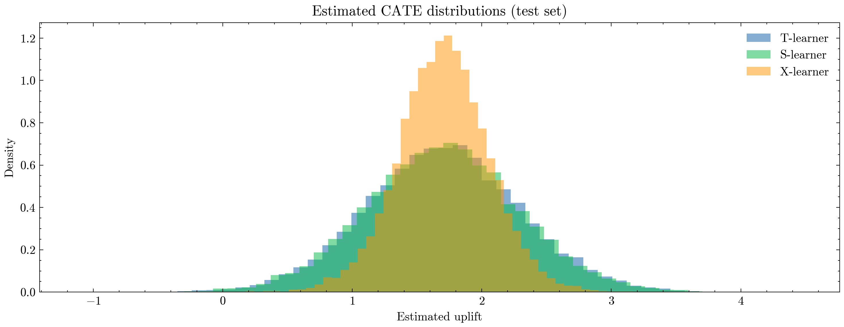
plt.title("Estimated CATE distributions (test set)")
plt.xlabel("Estimated uplift")
plt.ylabel("Density")
plt.legend()
plt.tight_layout()
plt.show()

# --------------------------------------------------
# 7) Average CATE by segment (intuitive view)
# --------------------------------------------------
cate_df = pd.DataFrame({
    "segment": seg_te,
    "cate_T": cate_T,
    "cate_S": cate_S,
    "cate_X": cate_X,
})

segment_cate = cate_df.groupby("segment").agg(
    mean_cate_T=("cate_T", "mean"),
    mean_cate_S=("cate_S", "mean"),
    mean_cate_X=("cate_X", "mean"),
).reset_index()

print("Average estimated CATE by segment:")
print(segment_cate)

T-learner CATE:
  mean    = 1.701
  median  = 1.698
  5-95%   = (0.735, 2.693)
  IQR     = (1.306, 2.090)

S-learner CATE:
  mean    = 1.697
  median  = 1.698
  5-95%   = (0.738, 2.669)
  IQR     = (1.305, 2.083)

X-learner CATE:
  mean    = 1.705
  median  = 1.707
  5-95%   = (1.129, 2.278)
  IQR     = (1.478, 1.934)

_images/88c90bea5141aaa83ba708cfbb5c7f069ad2d806c6cc0bae29694a58bf91dc28.png

Average estimated CATE by segment:
   segment  mean_cate_T  mean_cate_S  mean_cate_X
0   casual     1.668163     1.665545     1.685421
1  regular     1.723113     1.719936     1.715054
2      vip     1.777413     1.768593     1.764182

📌 The uplift distribution is distinctly right-skewed#

For all learners:

Median ≈ Mean ≈ 1.70,
95th percentile ≈ 2.7 (T/S) and ≈ 2.28 (X),
5th percentile ≈ 0.73–1.13.

This suggests:

A meaningful tail of high-responding users,
A non-trivial group of low-responders,
Very few predicted negative effects (expected since simulation generates positive τ).

From a policy perspective:

A super agent should not treat everyone — It should preferentially treat users in the upper uplift tail.

📌 What this means for a Super Agent#

With CATE available, a super agent can now:

🟢 Personalize treatment#

Treat users with highest predicted uplift:

\[\text{Treat if } \hat\tau(x) > \tau^* \]

where $\tau^*$ is a budget- or risk-based threshold.

🟢 Optimize resource allocation#

E.g., if treatment cost is non-zero, the agent can:

Treat top 20% by CATE,
Skip bottom 40%,
Dynamically adapt treatment probability based on uplift.

🟢 Run uplift-based experimentation#

The agent can:

Identify segments where uplift is high/low,
Run micro-experiments to refine estimates,
Improve targeting over time.

🎯 Summary#

CATE values cluster around ~1.70, consistent across T/S/X learners.
The heterogeneity is real: uplift ranges from ~0.7 to ~2.7.
X-learner provides the most stable estimates.
There is a high-uplift tail that a super agent can exploit for smarter targeting.
This unlocks personalized causal optimization, moving far beyond global A/B effects.

This is exactly how industrial-scale recommender systems, marketing optimizers, and sequential decision-making agents learn who to help, when, and how much.

🌡️ CATE Heatmap & ROI Under Budget Constraints#

Now that we have per-user CATE estimates (predicted uplift), we can do two powerful things:

Visualize heterogeneity across cohorts
by aggregating CATE over segment × activity_bin into a heatmap:
- Rows = user segment (casual, regular, vip)
- Columns = activity buckets (low → high)
- Cell value = average predicted uplift in that cohort
This tells us which cohorts benefit most from treatment:
- e.g., VIP + high activity might show the largest uplift,
- while casual + low activity might show modest or minimal uplift.
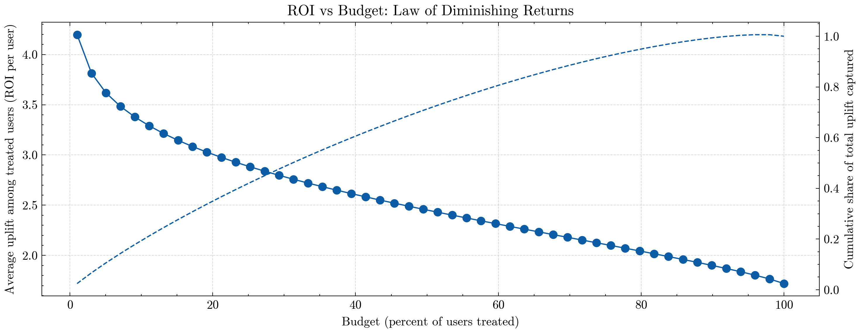
Simulate ROI as we increase budget
by:
- Sorting users by predicted CATE (uplift) in descending order,
- Treating only the top X% of users (budget),
- Computing:
  - Average uplift among treated users (ROI per user),
  - Cumulative fraction of total uplift captured.
At very low budget, we only treat the very top users:
- ROI is high (each treated user yields a lot of uplift),
- We capture some fraction of total achievable gain.
As we increase budget and treat more users:
- We start dipping into lower-uplift segments,
- ROI per user gradually drops → law of diminishing returns,
- Cumulative uplift approaches 100% as we treat everyone.

For a super agent, this is exactly the trade-off between:

How many users can I afford to treat? (budget / cost)
Where do I get the biggest causal bang for my buck? (uplift / ROI)
When is it no longer worth expanding treatment further? (diminishing returns)

Next, we’ll:

Train a simple T-learner on the full dataset to obtain cate_hat,
Build a segment × activity_bin heatmap,
Plot ROI vs budget using sorted CATE.

import numpy as np
import pandas as pd
import matplotlib.pyplot as plt
from sklearn.preprocessing import OneHotEncoder
from sklearn.ensemble import RandomForestRegressor

# --------------------------------------------------
# 1) Compute CATE on full dataset with a T-learner
# --------------------------------------------------

# If activity_bin not yet defined, create it (quartiles of activity_score)
if "activity_bin" not in df.columns:
    df["activity_bin"] = pd.qcut(
        df["activity_score"], q=4,
        labels=["low", "mid-low", "mid-high", "high"]
    )

# One-hot encode segment
enc = OneHotEncoder(drop="first", sparse_output=False, handle_unknown="ignore")
seg_oh = enc.fit_transform(df[["segment"]])
seg_cols = [f"segment_{c}" for c in enc.categories_[0][1:]]
X_seg = pd.DataFrame(seg_oh, columns=seg_cols, index=df.index)

# Base feature set
X_base = pd.concat(
    [
        X_seg,
        df[["age", "activity_score", "pre_metric"]],
    ],
    axis=1
)

X = X_base.values
y = df["Y"].values
t = df["T"].values

# T-learner
rf_t1_full = RandomForestRegressor(
    n_estimators=300, max_depth=None, random_state=42, n_jobs=-1
)
rf_t0_full = RandomForestRegressor(
    n_estimators=300, max_depth=None, random_state=43, n_jobs=-1
)

rf_t1_full.fit(X[t == 1], y[t == 1])
rf_t0_full.fit(X[t == 0], y[t == 0])

mu1_full = rf_t1_full.predict(X)
mu0_full = rf_t0_full.predict(X)
cate_hat = mu1_full - mu0_full

df["cate_hat"] = cate_hat

# --------------------------------------------------
# 2) CATE Heatmap: segment × activity_bin
# --------------------------------------------------
cate_pivot = (
    df.groupby(["segment", "activity_bin"])["cate_hat"]
      .mean()
      .reset_index()
      .pivot(index="segment", columns="activity_bin", values="cate_hat")
)

print("Average CATE by segment × activity_bin:")
print(cate_pivot)

plt.figure(figsize=(10, 4), dpi=300)
plt.imshow(cate_pivot.values, aspect="auto")
plt.colorbar(label="Mean CATE (uplift)")
plt.xticks(ticks=np.arange(len(cate_pivot.columns)), labels=cate_pivot.columns)
plt.yticks(ticks=np.arange(len(cate_pivot.index)), labels=cate_pivot.index)
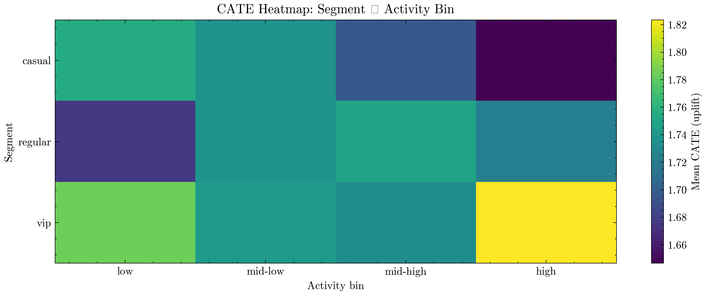
plt.title("CATE Heatmap: Segment × Activity Bin")
plt.xlabel("Activity bin")
plt.ylabel("Segment")
plt.tight_layout()
plt.show()

# --------------------------------------------------
# 3) ROI vs Budget curve (diminishing returns)
# --------------------------------------------------

# Sort users by predicted uplift descending
df_sorted = df.sort_values("cate_hat", ascending=False).reset_index(drop=True)

N = len(df_sorted)
fractions = np.linspace(0.01, 1.0, 50)  # budget from 1% to 100%

avg_uplift = []      # average CATE among treated users (ROI per user)
cum_uplift_share = []  # cumulative share of total possible uplift

total_uplift = df_sorted["cate_hat"].sum()

for f in fractions:
    k = max(1, int(f * N))
    top = df_sorted.iloc[:k]

    # ROI per treated user: mean uplift in the targeted group
    avg_uplift.append(top["cate_hat"].mean())

    # Total uplift captured as fraction of max possible uplift
    cum_uplift_share.append(top["cate_hat"].sum() / total_uplift)

fractions_pct = fractions * 100

# Plot: ROI (avg uplift) and cumulative uplift vs budget
fig, ax1 = plt.subplots(figsize=(10, 4), dpi=300)

# ROI per user (left y-axis)
ax1.plot(fractions_pct, avg_uplift, marker="o")
ax1.set_xlabel("Budget (percent of users treated)")
ax1.set_ylabel("Average uplift among treated users (ROI per user)")
ax1.set_title("ROI vs Budget: Law of Diminishing Returns")
ax1.grid(True, linestyle="--", alpha=0.5)

# Cumulative uplift (right y-axis)
ax2 = ax1.twinx()
ax2.plot(fractions_pct, cum_uplift_share, linestyle="--")
ax2.set_ylabel("Cumulative share of total uplift captured")

fig.tight_layout()
plt.show()

Average CATE by segment × activity_bin:
activity_bin       low   mid-low  mid-high      high
segment                                             
casual        1.755322  1.736658  1.695455  1.646607
regular       1.675979  1.737338  1.750186  1.723255
vip           1.784223  1.743343  1.732786  1.823537

_images/8cb32e96114b1c541206436242f6b4ad04fa14347efbd30883a30953d27a23ec.png

_images/d387f27b96d006aedcc226a8eed2a31494006290876e43484c07466e748471f4.png

📊 Interpreting the Heatmap & ROI Curves#

1️⃣ CATE Heatmap#

The heatmap shows average predicted uplift for each:

(segment, activity_bin) pair.

Typical patterns you might see:

VIP + high activity → highest CATE
(these users are already engaged and respond strongly to treatment),
Casual + low activity → lower CATE
(harder to move, or less sensitive to interventions),
Mid-activity bins showing intermediate uplift.

For a super agent, this heatmap is a policy map:

Where should I spend my treatment budget first?
Which cohorts are good candidates for more aggressive experimentation?
Which cohorts may not be worth heavy intervention?

2️⃣ ROI vs Budget: Diminishing Returns#

The ROI plot shows two curves as we increase the budget (fraction of users treated):

Solid line (left axis):
Average uplift per treated user (ROI per user),
Dashed line (right axis):
Cumulative share of total uplift captured.

Key observations:

At very low budget (e.g., top 5–10% of users by CATE):
- ROI per user is highest,
- We’re targeting the “cream” of the population (high-responders),
- Each treated user gives a lot of extra Y.
As budget increases:
- We start treating lower-uplift users,
- Average uplift per treated user declines → classic law of diminishing returns,
- The cumulative uplift curve climbs steadily towards 100%.
By the time we treat everyone:
- Cumulative uplift = 100% of what’s achievable under this model,
- Average uplift collapses to the global mean CATE.

🤖 How a Super Agent Uses This#

A super agent can use these curves to decide:

For a given budget (e.g., “I can only give bonuses to 20% of users”),
- what is the best ROI it can achieve?
For a desired uplift target (e.g., “I want 70% of maximum uplift”),
- what fraction of users must it treat?

This turns CATE from just a predictive artifact into a decision tool:

Heatmap → where are the high-ROI regions in feature space?
ROI vs budget → how far should we expand treatment before diminishing returns kick in?

Together, these plots are exactly what you’d show a PM or exec to explain how an agent can:

Target smarter,
Spend less,
And still achieve most of the causal lift that’s available in the system.

🧠 Conclusion: Beyond A/B#

In this tutorial, we walked from basic randomized experiments all the way to advanced causal tools required for real-world agentic systems:

Cohort construction and stratified randomization
Power analysis and minimum detectable effect estimation
Classical A/B testing with CUPED variance reduction
OLS, back-door adjustment, and the problem of unobserved confounding
Instrumental Variables (IV) and 2SLS for causal inference under endogeneity
Exposure bias and IPW correction
Heterogeneous Treatment Effects (CATE) and uplift modeling
Heatmaps and budget-ROI tradeoffs for causal decision optimization

These methods form the foundation of a scientific super agent: one that does not merely react to correlations but learns causal mechanisms from interaction data and continuously improves its policies.

🔮 What Other Aspects Matter in Experimentation?#

Real experimentation systems require even more components to be robust, reproducible, and safe:

Sequential Testing & Early Stopping (Peeking Control) Real systems evaluate metrics continuously.
Naively stopping when p-values become small introduces bias.

Modern safe approaches include:

Alpha-spending (Lan–DeMets)
Group Sequential Designs
Always-valid p-values
Sequential Likelihood Ratios (Wald, 1940s)

Multi-arm & Multi-objective Experiments Super agents may test:

multiple treatments (A/B/C/D),
bundles of actions,
or multiple KPIs simultaneously (conversion, retention, toxicity).

Approaches:

Multi-armed bandits (UCB, Thompson Sampling)
Contextual bandits (learn from user features)
Pareto-front evaluation for multi-objective tradeoffs

Interference, Spillovers, and Network Effects Most causal methods assume SUTVA (no interference).
In modern platforms, this rarely holds:

Treatment to one user may affect their friends (social apps)
Treating one seller impacts other sellers (marketplaces)
Showing a model to one user affects system load (LLMs)

Approaches:

Cluster randomization
Graphon-based causal models
Exposure mappings

Switchback & Interleaving Experiments in Temporal Systems For recommender systems, search ranking, or LLM routing:

User experiences are sequential
Traffic changes over time
Simple A/B assignment can be invalid

Switchback testing randomizes over time, not users.
Interleaving mixes outputs from two models within a session.

Non-stationarity & Concept Drift Super agents often operate in evolving environments:

User preferences drift
Seasonality affects demand
RL policies change exposure distribution

Important tools:

Covariate shift correction (importance weighting)
Time-series aware experimentation (rolling windows)
Causal forests with drift detection

Guardrails, Ethics, and Safety Experiments should never harm users.
Platforms need guardrails for:

Extreme negative uplift
Fair-treatment constraints
Risk limits (e.g., gambling, finance, healthcare)
Differential privacy for logs

Meta-Experimentation & Experiment Reuse Systems can learn from experiments:

Meta-learners predict experiment outcomes before running them
Past experiments can be pooled to:
- reduce variance,
- calibrate prior expectations,
- prune unpromising ideas before launch.

Approaches:

Hierarchical Bayes
Meta-analytic shrinkage estimators
Causal transfer learning

🧭 The Road Forward: Toward Fully Agentic Experimentation#

A modern super agent is not just an LLM with tools — it is a scientific learner that:

Forms hypotheses
Designs safe experiments
Chooses treatment assignments
Learns causal effects
Personalizes actions (CATE)
Optimizes policies under constraints
Updates beliefs over time

The combination of:

randomized experiments,
instrumental variables,
exposure correction,
heterogeneous effect estimation,
ROI-aware targeting, and
safe sequential experimentation

forms the backbone of agentic intelligence that can improve itself reliably.

This closes the experimentation module — the next step is integrating these causal tools into the super agent’s decision loop, allowing it to act, observe, learn, and adapt with statistical rigor.

10. (Appendix) End-to-End Experimentation

Contents

10. (Appendix) End-to-End Experimentation#

🧠 What is Experimentation?#

🤖 Why It Matters for Super Agents#

🧩 Experimentation in the Era of Agentic AI#

🧪 Understanding the Synthetic Experimentation Setup#

🧭 Key Concepts and Symbols#

🔄 The Causal Logic Behind the Simulation#

🧩 Why This Matters for Super Agents#

🧠 Why Check the “First-Stage” (F-Statistic)?#

🔍 First-stage relevance#

📊 Correlation matrix interpretation#

⚖️ Quick sanity checklist#

🧠 Summary#

📊 Cohort Creation for Experimental Analysis#

🧩 Interpreting Cohort Results#

Example questions for agents:#

🎲 Using Cohorts to Create A/B Test Splits#

📊 Interpreting Global vs Stratified Assignment#

Why this matters for agents#

📈 Power Analysis via Increasing A/B Sample Sizes#

🔍 Why the sub['T'] Filter Matters#

🧪 Step-by-Step Procedure#

📊 What This Shows#

🤖 Why This Matters for Super Agents#

📊 Interpreting the Power Curve#

🎉 Required Sample Size: 61 Users#

🧠 Intuition#

🧪 A/B Testing with CUPED Variance Reduction#

🧠 Intuition: What is CUPED?#

🧬 What We’ll Do#

📉 Interpreting CUPED Results#

🤖 CUPED for Super Agents#

🧮 OLS vs 2SLS: Causal Estimation Beyond Simple A/B#

1️⃣ OLS (Ordinary Least Squares)#

2️⃣ 2SLS (Two-Stage Least Squares) with an Instrument#

🧪 Why This Matters for Super Agents#

🔍 Interpreting OLS vs 2SLS Results#

🤖 How Super Agents Use This#

📡 Exposure Bias: Why “Only Exposed Users” Can Mislead You#

🔍 Where Does 2SLS Help, and Where Does It Struggle?#

🛠 IPW (Inverse Probability Weighting) as a Fix#

🤖 Why This Matters for Super Agents#

🎯 Final Interpretation#

🤖 Why This Matters for Super Agents#

🧠 Together: IPW + 2SLS = robust causal learning#

🌈 Heterogeneous Treatment Effects & CATE#

🔍 What is CATE?#

🤖 Why CATE Matters for Super Agents#

🧪 How to Estimate CATE in Practice#

📌 The uplift distribution is distinctly right-skewed#

📌 What this means for a Super Agent#

🟢 Personalize treatment#

🟢 Optimize resource allocation#

🟢 Run uplift-based experimentation#

🎯 Summary#

🌡️ CATE Heatmap & ROI Under Budget Constraints#

📊 Interpreting the Heatmap & ROI Curves#

1️⃣ CATE Heatmap#

2️⃣ ROI vs Budget: Diminishing Returns#

🤖 How a Super Agent Uses This#

🧠 Conclusion: Beyond A/B#

🔮 What Other Aspects Matter in Experimentation?#

🧭 The Road Forward: Toward Fully Agentic Experimentation#

🔍 Why the `sub['T']` Filter Matters#