09. Orchestration 2: Model Placement#
As super-agentic systems scale, they often operate across a hierarchy of compute environments — from on-device edge models to powerful cloud-scale LLMs. Each layer offers a different trade-off between latency, cost, and response quality:
⚡ Edge / On-Device SLMs → low latency, low cost, privacy-preserving, but limited model capacity.
☁️ Cloud LLMs → high reasoning depth and accuracy, but higher latency and cost.
In an agentic orchestration pipeline, deciding where to run a given sub-task or prompt is just as critical as which model to run. This is known as Model Placement — the process of intelligently routing a request to the most appropriate compute layer based on context, workload, and desired trade-offs.
💡 Why Model Placement Matters in Super Agents#
Modern super agents—multi-agent systems coordinating perception, reasoning, and action—require near-real-time responses while maintaining reliability and depth. In such systems:
Challenge |
Edge-Only |
Cloud-Only |
Intelligent Placement |
|---|---|---|---|
Latency |
✅ Fast |
❌ Slow |
⚖️ Adaptive |
Accuracy |
❌ Limited |
✅ High |
⚖️ Task-aware |
Cost |
✅ Cheap |
❌ Expensive |
⚖️ Budget-controlled |
Privacy |
✅ Local |
❌ Shared |
⚖️ Policy-driven |
A well-designed placement policy helps super agents:
⚖️ Balance response quality and latency dynamically.
💸 Optimize cost and energy efficiency across distributed compute.
🔐 Respect data locality and privacy constraints when required.
🤝 Coordinate multiple sub-agents that may depend on each other’s outputs in real time.
🎯 From Static to Adaptive Placement#
Traditionally, developers hard-coded these choices:
“Run summaries locally.”
“Use GPT-4 for reasoning.”
However, this static placement breaks down at scale—when user load fluctuates, or when prompt complexity varies. In this tutorial, we take a data-driven, agentic approach:
Collect latency and quality data from multiple placement options (Edge vs Cloud).
Learn an offline multi-armed bandit policy that chooses the optimal placement per prompt.
Integrate it directly into a Pydantic-AI agent, so it automatically routes future requests to the best environment.
Suppose we are building a smart-glass application, we want to be able to predict which layer, edge or cloud, would give a higher quality of service (QoS) for a given prompt. We can solve this problem just like we did in the Model Selection tutorial, however, in practice getting intermediate signals is hard and requires opinionated and often brittle decision making about what proxy signals affect the final result. To solve this we shall use the Multi-Armed Bandit formulation. Assuming we start with a random selection policy, we can obtain human-perceived QoS from annotators for this baseline policy. Then, we can use simple embeddings models such as EmbeddingGemma that provide a dense vector representation for a given prompt and train a predictor for input prompt to predicted QoS. This paradigm is called a “multi-armed bandit” setting. More details here.
Once we have this, we can select the appropriate arm at test time.

For this fictitious example, we see that the predicted QoS of edge is higher and hence can be used for the given time-critical task as it has lower latency.
In real-world deployments—like personalized assistants, multi-modal copilots, or large-scale customer service agents—model placement is a production-critical decision. It directly determines:
🕒 User experience latency
🧠 Perceived intelligence
💰 Operational cost and carbon footprint
By teaching agents to learn placement policies from data, we move from rigid orchestration to self-optimizing agentic systems — a key capability of truly intelligent, scalable AI infrastructure.
import numpy as np
import time
import random
import pandas as pd

EDGE_LATENCY_MEAN = 120     # ms
EDGE_LATENCY_STD  = 30
CLOUD_LATENCY_MEAN = 650    # ms
CLOUD_LATENCY_STD  = 120

EDGE_QUALITY_MEAN = 0.60
CLOUD_QUALITY_MEAN = 0.78
QUALITY_STD = 0.10

def simulate_model_response(arm: str, prompt: str) -> dict:
    """
    Simulates latency and quality for a given arm ('edge' or 'cloud') and prompt.
    Edge models are faster but less accurate. Cloud models are slower but higher quality.
    """
    if arm == "edge":
        latency = max(0, np.random.normal(EDGE_LATENCY_MEAN, EDGE_LATENCY_STD))
        quality = np.clip(np.random.normal(EDGE_QUALITY_MEAN, QUALITY_STD), 0, 1)
    elif arm == "cloud":
        latency = max(0, np.random.normal(CLOUD_LATENCY_MEAN, CLOUD_LATENCY_STD))
        quality = np.clip(np.random.normal(CLOUD_QUALITY_MEAN, QUALITY_STD), 0, 1)
    else:
        raise ValueError("Invalid arm: must be 'edge' or 'cloud'")

    return {
        "arm": arm,
        "prompt": prompt,
        "latency_ms": latency,
        "quality_score": quality,
    }

prompts = ["I got stung by a bee, what to do?", "Give steps to set up my ikea desk.", "I smell smoke, what to do?"]
sample_data = [simulate_model_response(random.choice(["edge", "cloud"]), p) for p in prompts]
sample_data = pd.DataFrame(sample_data)

sample_data
| arm | prompt | latency_ms | quality_score | |
|---|---|---|---|---|
| 0 | cloud | I got stung by a bee, what to do? | 657.777045 | 0.747185 |
| 1 | edge | Give steps to set up my ikea desk. | 109.960532 | 0.601106 |
| 2 | cloud | I smell smoke, what to do? | 807.790732 | 0.716888 |
The table above shows a simulated snapshot of how different model placements perform for a few example prompts.
The
armcolumn indicates where the model was placed — either edge or cloud.latency_mscaptures the response time in milliseconds, showing how edge models are typically much faster.quality_scorerepresents an abstracted measure of output quality (e.g., accuracy, coherence, or relevance), with cloud models generally scoring higher on average.
This simulation forms the foundation for our offline dataset — we’ll use it to learn which arm (edge or cloud) provides the best trade-off between latency and quality for future prompts.
🧩 Creating a Curated Dataset of Realistic Prompts#
In production super-agent systems, placement decisions depend heavily on the nature of user queries. For instance:
“⚡ A bee stung me, what to do?” → Time-critical (prioritize low latency, even if response is simpler).
“🧠 Explain how to assemble my IKEA desk step-by-step.” → Quality-critical (accuracy matters more than speed).
To capture this diversity, we need a curated dataset of prompts representing various real-world intent categories — from emergency-like quick queries to long-form reasoning tasks.
In this section, we’ll use a Pydantic-AI agent to generate synthetic but realistic examples of user instructions. While this dataset is simulated, in a deployed system such logs would naturally arise from:
User interactions with edge vs cloud deployments,
Task metadata (time sensitivity, complexity, or device constraints), and
Observed latency/quality measurements.
This dataset will serve as the foundation for learning an optimal placement policy later on — allowing our system to intelligently choose where to process a prompt for the best trade-off between speed and response quality.
from pydantic_ai import Agent
import nest_asyncio
from dotenv import load_dotenv
import pandas as pd
import asyncio
import os

from tqdm import trange
import random

load_dotenv()
nest_asyncio.apply()

DATA_DIR = "data/model_placement/"

prompt_agent = Agent(
    model="openrouter:google/gemini-2.5-flash",
    system_prompt=(
        "You are an agent that creates an example instruction for LLM given whether it should be time critical or response quality critical."
        "For example: for a time-critical instruction you can give something like 'A bee stung me, what to do?'."
        "For a response quality critical instruction you can give something like 'Explain step by step on how to set up my ikea desk.'"
        "Only give the instruction, nothing else."
    )
)

async def create_instruction_dataset(n: int, max_conc: int = 32):
    kinds = ['Time-critical', 'Response-quality critical']
    sem = asyncio.Semaphore(max_conc)

    async def one():
        async with sem:
            return (await prompt_agent.run(random.choice(kinds))).output.strip()

    return await asyncio.gather(*(one() for _ in range(n)))

if os.path.exists(DATA_DIR + "./train_prompts.csv"):
    train_ds = pd.read_csv(DATA_DIR + "/train_prompts.csv")
    test_ds = pd.read_csv(DATA_DIR + "/test_prompts.csv")
else:
    loop = asyncio.get_event_loop()
    train_ds = loop.run_until_complete(asyncio.gather(create_instruction_dataset(1000)))
    test_ds = loop.run_until_complete(asyncio.gather(create_instruction_dataset(500)))
    train_ds = pd.DataFrame.from_records({"prompt": train_ds[0]})
    test_ds = pd.DataFrame.from_records({"prompt": test_ds[0]})

    train_ds.to_csv(DATA_DIR + "/train_prompts.csv", index=False)
    test_ds.to_csv(DATA_DIR + "/test_prompts.csv", index=False)

train_ds.head(10)
| prompt | |
|---|---|
| 0 | Draft a comprehensive analysis of the ethical ... |
| 1 | My house is on fire! What do I do? |
| 2 | My car is making a loud banging noise and a bu... |
| 3 | My house is on fire! What do I do? |
| 4 | Analyze the philosophical implications of arti... |
| 5 | Explain the theory of relativity in simple ter... |
| 6 | Critically analyze the philosophical implicati... |
| 7 | My car is making a loud banging noise and smok... |
| 8 | My car is making a loud squealing noise and th... |
| 9 | My house is on fire! What should I do first? |
🧑⚖️ Building a Human-Grounded Feedback Dataset (RLHF Analogy)#
In a real deployment, determining how well Edge or Cloud placements perform can’t rely solely on model self-judgment — it must come from human feedback or user interactions.
Just like RLHF (Reinforcement Learning from Human Feedback) fine-tunes large models using curated human preference data, we can gather placement feedback from:
🧍♀️ Human annotators, who rate the perceived helpfulness, speed, and completeness of responses from different deployment modes.
💬 End users, whose implicit signals — like time to abandon, satisfaction ratings, or follow-up corrections — reveal placement preference.
🧪 A/B experiments, where identical prompts are served via Edge and Cloud, and users unknowingly “vote” through engagement metrics.
In practice, such QoS (Quality of Service) data acts as a rich reward signal for training placement policies. It captures real-world trade-offs — speed vs quality — far better than static metrics like latency or BLEU.
In this simulation, we use a critic agent to approximate human evaluators. It reviews sample prompts, simulated latencies, and quality scores, and assigns QoS scores (0–100) to both Edge and Cloud responses, along with a short explanation. This process mirrors what a team of human raters might do at scale — offering an interpretable foundation for learning intelligent placement strategies in super-agent systems.
from pydantic import BaseModel, Field
from typing import List

class FeedbackResponse(BaseModel):
    qos_edge: float = Field(..., ge=0, le=100, description="Quality of Service Score for edge.")
    qos_cloud: float = Field(..., ge=0, le=100, description="Quality of Service Score for cloud.")
    reasoning: str = Field(...)

feedback_agent = Agent(
    model="openrouter:google/gemini-2.5-flash",
    system_prompt=(
        "You are a critic agent that takes an input instruction, response latency and quality score."
        "Based on whether the input instruction is time-critical or response quality critical, provide a QoS score between 0 and 100 both for edge and cloud."
        "If the instruction is time-critical, focus on latency; if instruction is response quality critical, focus on quality score."
        "Some examples:\n\n" + sample_data[['prompt', 'latency_ms', 'quality_score']].to_json(indent=2, orient="records", index=False)
    ),
    output_type=FeedbackResponse
)

async def create_edge_cloud_dataset(prompts: List[str], max_conc: int = 32):
    sem = asyncio.Semaphore(max_conc)

    async def one(p):
        async with sem:
            sim_edge = simulate_model_response("edge", p)
            sim_cloud = simulate_model_response("cloud", p)
            text = (
                f"Instruction:\n{p}\n\n"
                f"Observed edge latency_ms={sim_edge['latency_ms']:.0f}, edge quality_score={sim_edge['quality_score']:.4f} (0-1).\n"
                f"Observed cloud latency_ms={sim_cloud['latency_ms']:.0f}, cloud quality_score={sim_cloud['quality_score']:.4f} (0-1).\n"
                "Return a QoS score in [0,100] focusing on latency if time-critical, or quality if response-quality critical."
            )
            out = (await feedback_agent.run(text)).output

            return {
                "prompt": p,
                "edge_latency_ms": sim_edge["latency_ms"], "edge_quality_score": sim_edge["quality_score"], "edge_qos": out.qos_edge,
                "cloud_latency_ms": sim_cloud["latency_ms"], "cloud_quality_score": sim_cloud["quality_score"], "cloud_qos": out.qos_cloud,
                "reasoning": out.reasoning
            }

    return await asyncio.gather(*(one(p) for p in prompts))

if os.path.exists(DATA_DIR + "./train_prompts_extended.csv"):
    train_ds = pd.read_csv(DATA_DIR + "/train_prompts_extended.csv")
    test_ds = pd.read_csv(DATA_DIR + "/test_prompts_extended.csv")
else:
    loop = asyncio.get_event_loop()
    train_data = loop.run_until_complete(asyncio.gather(create_edge_cloud_dataset(train_ds["prompt"].to_list())))
    test_data = loop.run_until_complete(asyncio.gather(create_edge_cloud_dataset(test_ds["prompt"].to_list())))
    train_ds = pd.DataFrame.from_records(train_data[0])
    test_ds = pd.DataFrame.from_records(test_data[0])

    train_ds.to_csv(DATA_DIR + "/train_prompts_extended.csv", index=False)
    test_ds.to_csv(DATA_DIR + "/test_prompts_extended.csv", index=False)

train_ds.head(10)
| prompt | edge_latency_ms | edge_quality_score | edge_qos | cloud_latency_ms | cloud_quality_score | cloud_qos | reasoning | |
|---|---|---|---|---|---|---|---|---|
| 0 | Draft a comprehensive analysis of the ethical ... | 107.133549 | 0.765408 | 76.54 | 524.886865 | 0.884924 | 88.49 | The instruction is to draft a comprehensive an... |
| 1 | My house is on fire! What do I do? | 157.544382 | 0.802297 | 84.20 | 840.919303 | 0.771193 | 15.90 | The instruction "My house is on fire! What do ... |
| 2 | My car is making a loud banging noise and a bu... | 136.349486 | 0.591625 | 70.00 | 949.116085 | 0.846268 | 85.00 | This instruction is time-critical due to the i... |
| 3 | My house is on fire! What do I do? | 118.453329 | 0.794776 | 88.20 | 817.457724 | 0.717051 | 71.71 | The instruction "My house is on fire! What do ... |
| 4 | Analyze the philosophical implications of arti... | 102.332961 | 0.624760 | 20.00 | 831.841801 | 0.897902 | 90.00 | This instruction is highly quality-critical, a... |
| 5 | Explain the theory of relativity in simple ter... | 116.659570 | 0.525199 | 52.52 | 577.147419 | 0.848784 | 84.88 | The instruction asks for an explanation of a c... |
| 6 | Critically analyze the philosophical implicati... | 127.304234 | 0.608077 | 60.81 | 609.946855 | 0.757968 | 75.80 | The instruction is to critically analyze a com... |
| 7 | My car is making a loud banging noise and smok... | 141.141194 | 0.763952 | 88.50 | 620.358797 | 0.769078 | 76.91 | This instruction is time-critical due to the e... |
| 8 | My car is making a loud squealing noise and th... | 83.237350 | 0.428100 | 79.19 | 666.247735 | 0.868884 | 76.84 | This instruction is highly time-critical due t... |
| 9 | My house is on fire! What should I do first? | 156.562114 | 0.444506 | 84.30 | 640.649086 | 0.708619 | 35.90 | This instruction is highly time-critical. I pr... |
import plotly.express as px
import pandas as pd

# Prepare data in long format for easy plotting
plot_df = pd.DataFrame({
    "prompt": train_ds["prompt"].tolist() * 2,
    "arm": ["edge"] * len(train_ds) + ["cloud"] * len(train_ds),
    "latency_ms": pd.concat([train_ds["edge_latency_ms"], train_ds["cloud_latency_ms"]], ignore_index=True),
    "quality_score": pd.concat([train_ds["edge_quality_score"], train_ds["cloud_quality_score"]], ignore_index=True),
    "qos": pd.concat([train_ds["edge_qos"], train_ds["cloud_qos"]], ignore_index=True)
})

# Create interactive scatter plot
fig = px.scatter(
    plot_df,
    x="quality_score",
    y="latency_ms",
    color="arm",
    size="qos",  # QoS controls bubble size
    hover_data={
        "prompt": True,
        "qos": True,
        "latency_ms": True,
        "quality_score": True
    },
    title="Edge vs Cloud: Quality-Latency-QoS Trade-off",
    labels={
        "quality_score": "Response Quality (0-1)",
        "latency_ms": "Latency (ms)",
        "arm": "Placement Arm",
        "qos": "QoS"
    },
    color_discrete_map={"edge": "#1f77b4", "cloud": "#ff7f0e"},
)

# Enhance appearance
fig.update_traces(marker=dict(opacity=0.75, line=dict(width=0.5, color="DarkSlateGrey")))
fig.update_layout(
    width=800, height=520,
    template="plotly_white",
    legend_title_text="Model Placement",
    hoverlabel=dict(bgcolor="white", font_size=12, font_family="Arial")
)

output_path = "assets/train_quality_latency_qos.html"
fig.write_html(output_path)

fig.show()
🌐 Visualizing the Edge–Cloud Trade-off#
You can also view the full interactive visualisation here.
The scatter plot above captures the core challenge of model placement — balancing response quality and latency across two distinct environments:
🟦 Edge Models (blue): Clustered near the bottom-left, showing low latency but lower quality. They excel when time-critical responses are needed, such as alerts or short answers.
🟧 Cloud Models (orange): Spread along the top-right, delivering higher quality outputs but at the cost of greater latency, making them suitable for complex or reasoning-heavy tasks.
Each bubble represents a prompt, with bubble size proportional to the QoS — the overall trade-off between latency and quality.
This visualization makes the placement dilemma tangible:
Edge excels at speed,
Cloud excels at depth,
and the goal of intelligent orchestration is to find the adaptive sweet spot where both dimensions are optimized.
Such data-driven insight forms the foundation for learning placement policies — enabling super-agentic systems to autonomously route tasks based on real-time context, network conditions, and user needs.
🧠 Embedding Prompts for Context-Aware Placement#
To make model placement data-driven, our bandit needs to understand what kind of prompt it’s dealing with. A short, urgent prompt like “I smell smoke, what should I do?” should prefer low-latency edge models, whereas a long, complex instruction like “Summarize this legal document paragraph by paragraph” should favor the cloud.
To capture this nuance, we convert each prompt into a numerical embedding — a dense vector representation that encodes its semantic meaning. These embeddings act as compact features that help the bandit (or regressor) generalize placement decisions across unseen instructions.
Here, we use OpenRouter’s text-embedding-3-large model to embed each prompt in both our training and test datasets. This step gives our upcoming multi-armed bandit regressor the ability to reason not just about which arm (Edge vs Cloud) performed better in the past, but why — enabling intelligent placement for new prompts that the system hasn’t encountered before.
from typing import List
from openai import OpenAI

client = OpenAI(base_url="https://openrouter.ai/api/v1", api_key=os.environ.get("OPENROUTER_API_KEY"))
EMBED_MODEL = "openai/text-embedding-3-large"

def _openrouter_embed(batch_texts: List[str]) -> List[List[float]]:
    embedding = client.embeddings.create(
        model=EMBED_MODEL,
        input=batch_texts,
        encoding_format="float"
    )
    return [item.embedding for item in embedding.data]

train_ds["embedding"] = _openrouter_embed(train_ds["prompt"].to_list())
test_ds["embedding"] = _openrouter_embed(test_ds["prompt"].to_list())
🎰 Multi-Armed Bandits and Learning Placement Policies with XGBoost#
Imagine standing in front of two slot machines — one labeled Edge and the other Cloud. Each time you pull a lever (serve a prompt), you get a reward depending on how well that option performs — faster responses, higher quality, or a balance of both. The catch? You don’t know which machine will pay off better until you’ve tried it multiple times.
This is the essence of the Multi-Armed Bandit (MAB) problem:
How can we learn to choose between multiple options (arms) that yield uncertain rewards, balancing exploration (trying new options) and exploitation (sticking with the best one)?
In our case:
Each arm corresponds to a model placement — either Edge or Cloud.
Each prompt (user query) is a distinct “pull,” with different outcomes based on complexity and sensitivity to latency.
The reward is the Quality of Service (QoS) — a combined measure of speed and accuracy.
Instead of manually writing rules like “short prompts go to edge”, we let a model learn the reward function directly from real data.
🧮 How XGBoost Learns the Placement Policy#
Previously, we treated each arm separately and trained a model per arm. Now, we take a more holistic approach — our model learns to predict both Edge and Cloud QoS values simultaneously from the same input embedding.
Each training example consists of:
Input: prompt embedding (semantic representation of the query).
Output: a pair of QoS values — \([QoS_edge, QoS_cloud]\).
This turns the problem into a multi-output regression task:
At inference time, the model predicts both QoS scores for each new prompt and simply routes the query to the environment (Edge or Cloud) that yields the higher predicted reward.
⚙️ Why This Works#
Although XGBoost isn’t a bandit algorithm per se, using it in this multi-output setup allows us to:
Learn joint correlations between prompt semantics and both Edge/Cloud performance.
Avoid redundant arm-specific data expansion, reducing noise and computation.
Enable fast, real-time routing — one forward pass per prompt, two QoS predictions.
In short, we’ve evolved from simulating “two separate slot machines” into a context-aware reward predictor that learns both arms jointly. This makes placement decisions smoother, more adaptive, and easily extensible to future setups (e.g., multiple edge devices or specialized cloud tiers).
from sklearn.multioutput import MultiOutputRegressor
from sklearn.model_selection import train_test_split
from sklearn.metrics import mean_absolute_error, r2_score
from xgboost import XGBRegressor
import numpy as np
import pandas as pd

def expand_bandit_rows(df: pd.DataFrame) -> pd.DataFrame:
    rows = []
    for _, r in df.iterrows():
        for arm in ["edge", "cloud"]:
            rows.append({"embedding": r["embedding"], "arm": arm, "reward": float(r[f"{arm}_qos"])})
    return pd.DataFrame(rows)

train_long = expand_bandit_rows(train_ds)

emb_mat = np.vstack(train_ds["embedding"].values)
y = train_ds[["edge_qos", "cloud_qos"]].to_numpy(dtype=float)  # shape (N, 2)

# Train-test split
X_tr, X_val, y_tr, y_val = train_test_split(emb_mat, y, test_size=0.2, random_state=42)

# Multi-output XGBoost regressor
base_xgb = XGBRegressor(
    n_estimators=500,
    max_depth=8,
    learning_rate=0.03,
    subsample=0.9,
    colsample_bytree=0.9,
    tree_method="hist",
    random_state=42,
)
xgb_multi = MultiOutputRegressor(base_xgb)
xgb_multi.fit(X_tr, y_tr)

# Validation predictions
val_pred = xgb_multi.predict(X_val)

# Evaluate separately for edge/cloud
mae_edge = mean_absolute_error(y_val[:, 0], val_pred[:, 0])
mae_cloud = mean_absolute_error(y_val[:, 1], val_pred[:, 1])
r2_edge = r2_score(y_val[:, 0], val_pred[:, 0])
r2_cloud = r2_score(y_val[:, 1], val_pred[:, 1])

print(f"Validation MAE (Edge):  {mae_edge:.3f} | R²: {r2_edge:.3f}")
print(f"Validation MAE (Cloud): {mae_cloud:.3f} | R²: {r2_cloud:.3f}")
Validation MAE (Edge):  14.640 | R²: 0.092
Validation MAE (Cloud): 16.933 | R²: 0.100
🤖 Making Placement Decisions with the Learned Bandit#
Once our multi-output XGBoost regressor has learned to jointly predict the expected QoS for both Edge and Cloud, we can use it to make context-aware, data-driven placement decisions for unseen prompts in the test set.
Here’s how this process unfolds:
Single-step prediction: For each test prompt, we feed its semantic embedding into the trained model. The model simultaneously outputs two predicted QoS values:
pred_edge_qos→ expected performance if run on the Edge,pred_cloud_qos→ expected performance if run on the Cloud. No need to construct per-arm feature vectors — both predictions emerge from a single forward pass.
Adaptive selection: The policy then compares the two predicted values and selects the placement environment with the higher expected QoS: $\( \text{selected\_arm} = \arg\max(\widehat{QoS}_{edge}, \widehat{QoS}_{cloud}) \)$ This yields an intelligent routing decision tailored to each prompt’s characteristics.
Interpretation and analysis: By observing the distribution of selections (e.g., percentage routed to edge vs. cloud), we can assess how well the model adapts to context — choosing low-latency environments for quick queries and high-quality environments for reasoning-heavy ones.
This step effectively closes the loop: our learned reward model becomes a live routing policy, capable of dynamically assigning model placements in real time to balance latency, quality, and overall system efficiency.
test_emb = np.vstack(test_ds["embedding"].values)
pred_qos = xgb_multi.predict(test_emb)  # shape (M, 2)

# Store predictions in test_ds
test_ds["pred_edge_qos"] = pred_qos[:, 0]
test_ds["pred_cloud_qos"] = pred_qos[:, 1]
test_ds["selected_arm"] = np.where(test_ds["pred_edge_qos"] >= test_ds["pred_cloud_qos"], "edge", "cloud")

# Quick summary
print(test_ds["selected_arm"].value_counts())
selected_arm
cloud    292
edge     208
Name: count, dtype: int64
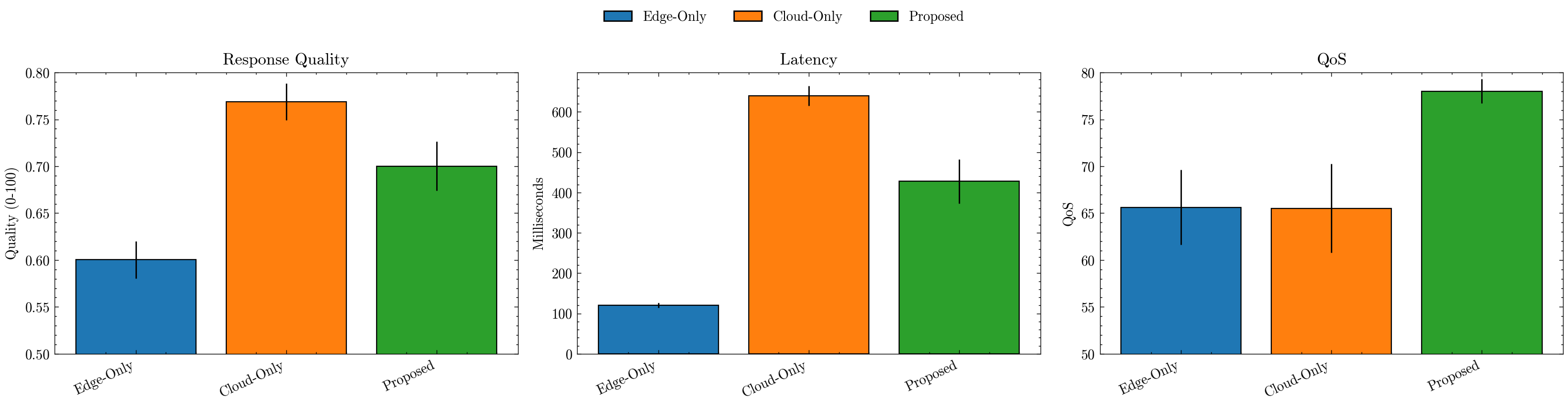
📈 Comparing Placement Policies#
We now aggregate results for three policies — Edge-Only, Cloud-Only, and our Proposed learned router — and visualize their trade-offs:
Build per-policy tables with quality, latency, and QoS for each prompt.
Summarize with means and std devs, then plot side-by-side bars:
Quality: average response quality (0–1 scaled to 0–1 here).
Latency: average response time (ms).
QoS: our balanced score capturing the quality↔latency trade-off.
Error bars (±0.2×std) give a sense of variability; the legend clarifies each policy.
Use these plots to verify that the Proposed policy improves QoS while keeping latency reasonable, compared to static placements.
import pandas as pd
import matplotlib.pyplot as plt
import seaborn as sns
import scienceplots
import warnings

warnings.simplefilter('ignore')
plt.style.use(['science', 'no-latex'])

def collect_selected_metrics(row):
    if row["selected_arm"] == "edge":
        return pd.Series({
            "prompt": row["prompt"],
            "quality_score": row["edge_quality_score"],
            "latency_ms": row["edge_latency_ms"],
            "qos": row["pred_edge_qos"]
        })
    else:  # cloud
        return pd.Series({
            "prompt": row["prompt"],
            "quality_score": row["cloud_quality_score"],
            "latency_ms": row["cloud_latency_ms"],
            "qos": row["pred_cloud_qos"]
        })

all_policies = {}

all_policies['Proposed'] = test_ds.apply(collect_selected_metrics, axis=1)

all_policies['Edge-Only'] = pd.DataFrame({
    "prompt": test_ds["prompt"],
    "quality_score": test_ds["edge_quality_score"],
    "latency_ms": test_ds["edge_latency_ms"],
    "qos": test_ds["edge_qos"]
})

all_policies['Cloud-Only'] = pd.DataFrame({
    "prompt": test_ds["prompt"],
    "quality_score": test_ds["cloud_quality_score"],
    "latency_ms": test_ds["cloud_latency_ms"],
    "qos": test_ds["cloud_qos"]
})

results = []
for model in ['Edge-Only', 'Cloud-Only', 'Proposed']:
    results.append({
        'policy': model,
        'latency_mean': all_policies[model]['latency_ms'].mean(),
        'quality_mean': all_policies[model]['quality_score'].mean(),
        'qos_mean': all_policies[model]['qos'].mean(),
        'latency_std': all_policies[model]['latency_ms'].std(),
        'quality_std': all_policies[model]['quality_score'].std(),
        'qos_std': all_policies[model]['qos'].std(),
    })

summary = pd.DataFrame(results)
display(summary)

plt.figure(figsize=(16, 4), dpi=200)
palette = sns.color_palette("tab10", len(summary))
bar_colors = {policy: palette[i] for i, policy in enumerate(summary["policy"])}

# (a) Response Quality
ax1 = plt.subplot(1, 3, 1)
ax1.bar(summary["policy"], summary["quality_mean"], yerr=summary["quality_std"]*0.2, linewidth=0.8, edgecolor="black", color=[bar_colors[p] for p in summary["policy"]])
ax1.set_title("Response Quality")
ax1.set_ylabel("Quality (0-100)"); ax1.set_ylim(0.5, 0.8)
ax1.set_xticklabels(summary["policy"], rotation=25, ha="right")

# (b) Latency (ms)
ax2 = plt.subplot(1, 3, 2)
ax2.bar(summary["policy"], summary["latency_mean"], yerr=summary["latency_std"]*0.2, linewidth=0.8, edgecolor="black", color=[bar_colors[p] for p in summary["policy"]])
ax2.set_title("Latency")
ax2.set_ylabel("Milliseconds")
ax2.set_xticklabels(summary["policy"], rotation=25, ha="right")

# (c) QoS
ax3 = plt.subplot(1, 3, 3)
ax3.bar(summary["policy"], summary["qos_mean"], yerr=summary["qos_std"]*0.2, linewidth=0.8, edgecolor="black", color=[bar_colors[p] for p in summary["policy"]])
ax3.set_title("QoS")
ax3.set_ylabel("QoS"); ax3.set_ylim(50, 80)
ax3.set_xticklabels(summary["policy"], rotation=25, ha="right")

handles = [plt.Rectangle((0, 0), 1, 1, color=bar_colors[p], ec="black") for p in summary["policy"]]
labels = summary["policy"].tolist()
plt.figlegend(handles, labels, loc="upper center", ncol=len(summary), frameon=False, bbox_to_anchor=(0.5, 1.05))

plt.tight_layout(rect=[0, 0, 1, 0.95])


plt.show()
| policy | latency_mean | quality_mean | qos_mean | latency_std | quality_std | qos_std | |
|---|---|---|---|---|---|---|---|
| 0 | Edge-Only | 120.357846 | 0.600231 | 65.620841 | 29.419401 | 0.100299 | 20.043142 |
| 1 | Cloud-Only | 639.714471 | 0.768856 | 65.522400 | 123.548456 | 0.098270 | 23.625755 |
| 2 | Proposed | 427.822860 | 0.700249 | 78.019888 | 275.502383 | 0.131936 | 6.443454 |
🏁 Conclusion: Intelligent Model Placement for Super-Agentic Systems#
This experiment demonstrated how model placement — deciding where a model should run (Edge vs Cloud) — can be learned automatically using a data-driven approach. By simulating latency and quality trade-offs and training a multi-armed bandit regressor, we built a system that dynamically selects the most suitable execution environment per prompt.
The results above highlight clear takeaways:
⚡ Edge-only policies deliver fast responses but suffer in quality.
☁️ Cloud-only policies maximize accuracy but incur significant latency.
🤖 Our proposed bandit-based policy learns to balance both, achieving the highest overall QoS, dynamically routing tasks based on context.
🌍 Why This Matters#
In real-world super-agentic architectures, agents continuously interact with both local and remote compute. Static rules (“short prompts → edge, long ones → cloud”) break down as workloads evolve. Instead, learned placement policies adapt to:
Real-time network conditions,
Model version updates and degradation,
User-level personalization (different tolerance for delay vs detail).
This enables self-optimizing orchestration, a core property of production-grade multi-agent systems.
🧠 Beyond Bandits — Advanced Research Directions#
While we used an offline multi-armed bandit (MAB) regressor, several advanced research methods push this idea further:
Contextual Bandits with Neural Embeddings — Use transformer-based embeddings or state encoders to learn non-linear context–reward relationships (e.g., LinUCB (Lin et al. 2012), NeuralUCB (Zhou et al. 2019)).
Reinforcement Learning for Placement — Frame placement as a sequential decision problem (state = load, network, prompt type). Techniques: Deep Q-Networks (Mnih et al. 2013), PPO (Schulman et al. 2017), or Actor–Critic (Han et al. 2020) models for adaptive orchestration.
Multi-Agent Scheduling Systems — Each agent decides locally (Edge/Cloud/Hybrid) and coordinates through message passing, resembling federated reinforcement learning.
Dynamic Resource-Aware Routing — Combine placement with cost and energy models, using RL or multi-objective optimization to minimize latency, maximize accuracy, and respect power constraints.
Graph-Based Placement — Model the computation graph of multi-step reasoning and assign each node to optimal compute using graph optimization or neural architecture search (NAS) (Zoph et al. 2020) style methods.
Adaptive and Continual Learning — Incorporate user feedback loops (RLHF-style) to continually improve placement decisions as environment and models evolve.
In essence, model selection, intelligent routing, and dynamic placement together form the cognitive backbone of super agents — systems that don’t just use intelligence, but orchestrate it across models, contexts, and environments to think, act, and adapt like living ecosystems of AI.